Lecture 1: Floating-point arithmetic, vector norms
Syllabus
Today:
- Part 1: floating point, vector norms
- Part 2: matrix norms and stability concepts
Tomorrow: Matrix norms and unitary matrices
Representation of numbers
- Real numbers represent quantities: probabilities, velocities, masses, ...

- It is important to know, how they are represented in the computer, which only knows about bits.
Fixed point
The most straightforward format for the representation of real numbers is fixed point representation, also known as Qm.n format.
A Qm.n number is in the range $[-(2^m), 2^m - 2^{-n}]$, with resolution $2^{-n}$.
Total storage is $m + n + 1$ bits.
The range of numbers represented is fixed.
Floating point
The numbers in computer memory are typically represented as floating point numbers
A floating point number is represented as
$$\textrm{number} = \textrm{significand} \times \textrm{base}^{\textrm{exponent}},$$where significand is integer, base is positive integer and exponent is integer (can be negative), i.e.
$$ 1.2 = 12 \cdot 10^{-1}.$$- This format has a long history. It was already used in the world's first working programmable, fully automatic digital computer Z3) designed in 1935 and completed in 1941 in Germany by Konrad Zuse.
Floating point: formula
$$f = (-1)^s 2^{(p-b)} \left( 1 + \frac{d_1}{2} + \frac{d_2}{2^2} + \ldots + \frac{d_m}{2^m}\right),$$where $s \in \{0, 1\}$ is the sign bit, $d_i \in \{0, 1\}$ is the $m$-bit mantissa, $p \in \mathbb{Z}; 0 \leq p \leq 2^e$, $e$ is the $e$-bit exponent, commonly defined as $2^e - 1$
Can be thought as a uniform $m$-bit grid between two sequential powers of $2$.
Fixed vs Floating
Q: What are the advantages/disadvantages of the fixed and floating points?
A: In most cases, they work just fine.
However, fixed point represents numbers within specified range and controls absolute accuracy.
Floating point represent numbers with relative accuracy, and is suitable for the case when numbers in the computations have varying scale (i.e., $10^{-1}$ and $10^{5}$).
In practice, if speed is of no concern, use float32 or float64.
IEEE 754
In modern computers, the floating point representation is controlled by IEEE 754 standard which was published in 1985 and before that point different computers behaved differently with floating point numbers.
IEEE 754 has:
- Floating point representation (as described above), $(-1)^s \times c \times b^q$.
- Two infinities, $+\infty$ and $-\infty$
- Two zeros: +0 and -0
- Two kinds of NaN: a quiet NaN (qNaN) and signalling NaN (sNaN)
- qNaN does not throw exception in the level of floating point unit (FPU), until you check the result of computations
- sNaN value throws exception from FPU if you use corresponding variable. This type of NaN can be useful for initialization purposes
- C++11 proposes standard interface for creating different NaNs
- Rules for rounding
- Rules for $\frac{0}{0}, \frac{1}{-0}, \ldots$
Possible values are defined with
- base $b$
- accuracy $p$ - number of digits
- maximum possible value $e_{\max}$
and have the following restrictions
- $ 0 \leq c \leq b^p - 1$
- $1 - e_{\max} \leq q + p - 1 \leq e_{\max}$
The two most common format, single & double
The two most common formats, called binary32 and binary64 (called also single and double formats). Recently, the format binary16 plays important role in learning deep neural networks.
| Name | Common Name | Base | Digits | Emin | Emax |
|---|---|---|---|---|---|
| binary16 | half precision | 2 | 11 | -14 | + 15 |
| binary32 | single precision | 2 | 24 | -126 | + 127 |
| binary64 | double precision | 2 | 53 | -1022 | +1023 |
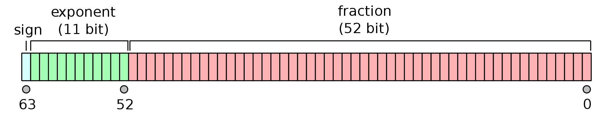
Examples
- For a number +0
- sign is 0
- exponent is 00000000000
- fraction is all zeros
- For a number -0
- sign is 1
- exponent is 00000000000
- fraction is all zeros
- For +infinity
- sign is 0
- exponent is 11111111111
- fraction is all zeros
Q: what about -infinity and NaN ?
Accuracy and memory
The relative accuracy of single precision is $10^{-7}-10^{-8}$, while for double precision is $10^{-14}-10^{-16}$.
Crucial note 1: A float16 takes 2 bytes, float32 takes 4 bytes, float64, or double precision, takes 8 bytes.
Crucial note 2: These are the only two floating point-types supported in hardware (float32 and float64) + GPU/TPU different float types are supported.
Crucial note 3: You should use double precision in computational science and engineering and float on GPU/Data Science.
Also, half precision can be useful in training deep neural network, see this paper.
How does number representation format affect training of neural networks (NN)?
- Weights in layers (fully-connected, convolutional, activation functions) can be stored with different accuracies
- It is important to improve energy efficiency of the devices that are used to train NNs
- Project DeepFloat from Facebook demonstrates how re-develop floating point operations in a way to ensure efficiency in training NNs, more details see in this paper
- Affect of the real numbers representation on the gradients of activation functions
- Typically, the first digit is one.
- Subnormal numbers have first digit 0 to represent zeros and numbers close to zero.
- Subnormal numbers fill the gap between positive and negative
- They have performance issues, often flushed to zero by default.
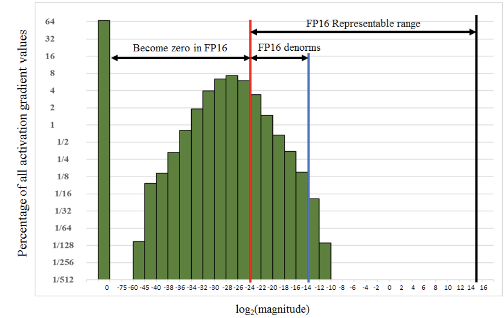
- And on the learning curves
Plots are taken from this paper
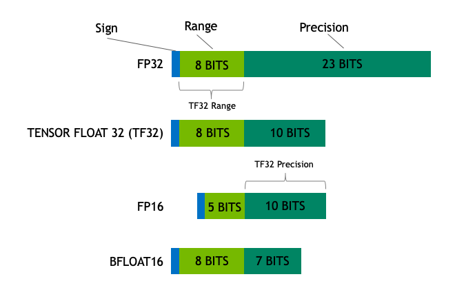
bfloat16 (Brain Floating Point)
- This format occupies 16 bits
- 1 bit for sign
- 8 bits for exponent
- 7 bits for fraction
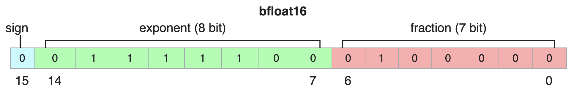
- Truncated single precision format from IEEE standard
- What is the difference between float32 and float16?
- This format is utilized in Intel FPGA, Google TPU, Xeon CPUs and other platforms
Tensor Float from Nvidia (blog post about this format)
- Comparison with other formats
- Results

- PyTorch and Tensorflow supported this format are available in Nvidia NCG
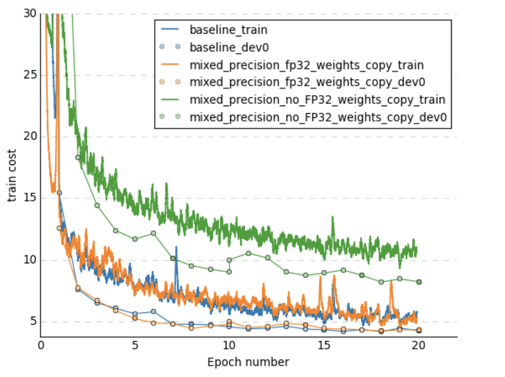
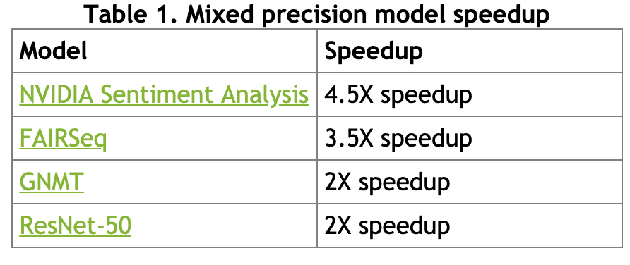
Mixed precision (docs from Nvidia)
- Main idea:
- Maintain copy of weights in single precision
- Then in every iteration
- Make a copy of weights in half-precision
- Forward pass with weights in half-precision
- Multiply the loss by the scaling factor $S$
- Backward pass again in half precision
- Multiply the weight gradient with $1/S$
- Complete the weight update (including gradient clipping, etc.)
- Scaling factor $S$ is a hyper-parameter
- Constant: a value so that its product with the maximum absolute gradient value is below 65504 (the maximum value representable in half precision).
- Dynamic update based on the current gradient statistics
Performance comparison
Automatic mixed-precision extensions exist to simplify turning this option on, more details here
Alternative to the IEEE 754 standard
Issues in IEEE 754:
- overflow to infinity or zero
- many different NaNs
- invisible rounding errors
- accuracy is very high or very poor
- subnormal numbers – numbers between 0 and minimal possible represented number, i.e. significand starts from zero
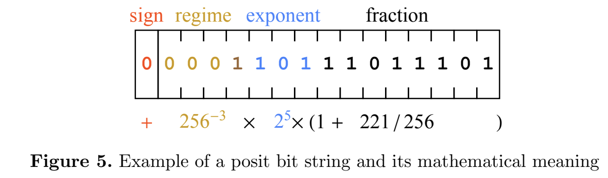
Concept of posits can replace floating point numbers, see this paper
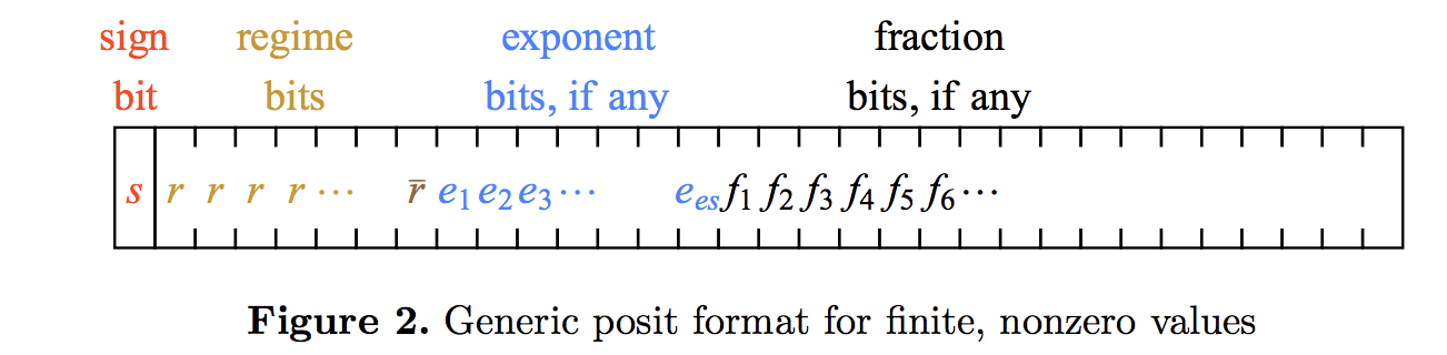
- represent numbers with some accuracy, but provide limits of changing
- no overflows!
- example of a number representation
Division accuracy demo
import random
import jax.numpy as jnp
import jax
from jax.config import config
config.update("jax_enable_x64", True)
#c = random.random()
#print(c)
c = jnp.float32(0.925924589693)
print(c)
a = jnp.float32(1e-50)
b = jnp.float32(c / a)
print('{0:10.16f}'.format(b))
print(abs(a * b - c)/abs(c))
0.9259246
       inf
nan
Square root accuracy demo
a = jnp.float32(1e-40)
b = jnp.sqrt(a)
print(b.dtype)
print('{0:10.64f}'.format(abs(b * b - a)/abs(a)))
float32
       nan
Exponent accuracy demo
a = jnp.float32(1e99)
b = jnp.exp(a)
print(b.dtype)
print(jnp.log(b) - a)
float32
nan
Loss of significance
- Many operations lead to the loss of digits loss of significance
- For example, it is a bad idea to subtract two big numbers that are close, the difference will have fewer correct digits
- This is related to algorithms and their properties (forward/backward stability), which we will discuss later
Summation algorithm
However, the rounding errors can depend on the algorithm.
Consider the simplest problem: given $n$ floating point numbers $x_1, \ldots, x_n$
Compute their sum
The simplest algorithm is to add one-by-one
What is the actual error for such algorithm?
Naïve algorithm
Naïve algorithm adds numbers one-by-one:
$$y_1 = x_1, \quad y_2 = y_1 + x_2, \quad y_3 = y_2 + x_3, \ldots.$$The worst-case error is then proportional to $\mathcal{O}(n)$, while mean-squared error is $\mathcal{O}(\sqrt{n})$.
The Kahan algorithm gives the worst-case error bound $\mathcal{O}(1)$ (i.e., independent of $n$).
Can you find the better algorithm?
Kahan summation
The following algorithm gives $2 \varepsilon + \mathcal{O}(n \varepsilon^2)$ error, where $\varepsilon$ is the machine precision.
- The reason of the loss of significance in summation is operating with numbers of different magnitude
- The main idea of Kahan summation is to keep track of small errors and aggregate them in separate variable
- This approach is called compensated summation
s = 0
c = 0
for i in range(len(x)):
    y = x[i] - c
    t = s + y
    c = (t - s) - y
    s = t
- There exists more advanced tricks to process this simple operation that are used for example in
fsumfunction frommathpackage, implementation check out here
import math

import jax.numpy as jnp
import numpy as np
import jax
from numba import jit as numba_jit

n = 10 ** 7
sm = 1e-10
x = jnp.ones(n, dtype=jnp.float32) * sm
x = x.at[0].set(1)
#x = jax.ops.index_update(x, [0], 1.)
true_sum = 1.0 + (n - 1)*sm
approx_sum = jnp.sum(x)
math_fsum = math.fsum(x)


@jax.jit
def dumb_sum(x):
    s = jnp.float32(0.0)
    def b_fun(i, val):
        return val + x[i]
    s = jax.lax.fori_loop(0, len(x), b_fun, s)
    return s


@numba_jit(nopython=True)
def kahan_sum_numba(x):
    s = np.float32(0.0)
    c = np.float32(0.0)
    for i in range(len(x)):
        y = x[i] - c
        t = s + y
        c = (t - s) - y
        s = t
    return s

@jax.jit
def kahan_sum_jax(x):
    s = jnp.float32(0.0)
    c = jnp.float32(0.0)
    def b_fun2(i, val):
        s, c = val
        y = x[i] - c
        t = s + y
        c = (t - s) - y
        s = t
        return s, c
    s, c = jax.lax.fori_loop(0, len(x), b_fun2, (s, c))
    return s

k_sum_numba = kahan_sum_numba(np.array(x))
k_sum_jax = kahan_sum_jax(x)
d_sum = dumb_sum(x)
print('Error in np sum: {0:3.1e}'.format(approx_sum - true_sum))
print('Error in Kahan sum Numba: {0:3.1e}'.format(k_sum_numba - true_sum))
print('Error in Kahan sum JAX: {0:3.1e}'.format(k_sum_jax - true_sum))
print('Error in dumb sum: {0:3.1e}'.format(d_sum - true_sum))
print('Error in math fsum: {0:3.1e}'.format(math_fsum - true_sum))
Error in np sum: -8.3e-07
Error in Kahan sum Numba: 4.7e-08
Error in Kahan sum JAX: 0.0e+00
Error in dumb sum: -1.0e-03
Error in math fsum: 1.3e-11
More complicated example
import math
test_list = [1, 1e20, 1, -1e20]
print(math.fsum(test_list))
print(jnp.sum(jnp.array(test_list, dtype=jnp.float32)))
print(1 + 1e20 + 1 - 1e20)
2.0
0.0
0.0
Summary of floating-point
You should be really careful with floating point numbers, since it may give you incorrect answers due to rounding-off errors.
For many standard algorithms, the stability is well-understood and problems can be easily detected.
Vectors
- In NLA we typically work not with numbers, but with vectors
- Recall that a vector in a fixed basis of size $n$ can be represented as a 1D array with $n$ numbers
- Typically, it is considered as an $n \times 1$ matrix (column vector)
Example: Polynomials with degree $\leq n$ form a linear space. Polynomial $ x^3 - 2x^2 + 1$ can be considered as a vector $\begin{bmatrix}1 \\ -2 \\ 0 \\ 1\end{bmatrix}$ in the basis $\{x^3, x^2, x, 1\}$
Vector norm
Vectors typically provide an (approximate) description of a physical (or some other) object
One of the main question is how accurate the approximation is (1%, 10%)
What is an acceptable representation, of course, depends on the particular applications. For example:
- In partial differential equations accuracies $10^{-5} - 10^{-10}$ are the typical case
- In data-based applications sometimes an error of $80\%$ is ok, since the interesting signal is corrupted by a huge noise
Distances and norms
- Norm is a qualitative measure of smallness of a vector and is typically denoted as $\Vert x \Vert$.
The norm should satisfy certain properties:
- $\Vert \alpha x \Vert = |\alpha| \Vert x \Vert$
- $\Vert x + y \Vert \leq \Vert x \Vert + \Vert y \Vert$ (triangle inequality)
- If $\Vert x \Vert = 0$ then $x = 0$
The distance between two vectors is then defined as
$$ d(x, y) = \Vert x - y \Vert. $$Standard norms
The most well-known and widely used norm is euclidean norm:
$$\Vert x \Vert_2 = \sqrt{\sum_{i=1}^n |x_i|^2},$$which corresponds to the distance in our real life. If the vectors have complex elements, we use their modulus.
$p$-norm
Euclidean norm, or $2$-norm, is a subclass of an important class of $p$-norms:
$$ \Vert x \Vert_p = \Big(\sum_{i=1}^n |x_i|^p\Big)^{1/p}. $$There are two very important special cases:
- Infinity norm, or Chebyshev norm is defined as the element of the maximal absolute value:

- $L_1$ norm (or Manhattan distance) which is defined as the sum of modules of the elements of $x$:
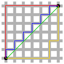
We will give examples where $L_1$ norm is very important: it all relates to the compressed sensing methods that emerged in the mid-00s as one of the most popular research topics.
Equivalence of the norms
All norms are equivalent in the sense that
$$ C_1 \Vert x \Vert_* \leq \Vert x \Vert_{**} \leq C_2 \Vert x \Vert_* $$for some positive constants $C_1(n), C_2(n)$, $x \in \mathbb{R}^n$ for any pairs of norms $\Vert \cdot \Vert_*$ and $\Vert \cdot \Vert_{**}$. The equivalence of the norms basically means that if the vector is small in one norm, it is small in another norm. However, the constants can be large.
Computing norms in Python
The NumPy package has all you need for computing norms: np.linalg.norm function.
n = 100
a = jnp.ones(n)
b = a + 1e-3 * jax.random.normal(jax.random.PRNGKey(0), (n,))
print('Relative error in L1 norm:', jnp.linalg.norm(a - b, 1) / jnp.linalg.norm(b, 1))
print('Relative error in L2 norm:', jnp.linalg.norm(a - b) / jnp.linalg.norm(b))
print('Relative error in Chebyshev norm:', jnp.linalg.norm(a - b, jnp.inf) / jnp.linalg.norm(b, jnp.inf))
Relative error in L1 norm: 0.0008608277121789923
Relative error in L2 norm: 0.0010668749128008221
Relative error in Chebyshev norm: 0.0025285461541625647
Unit disks in different norms
- A unit disk is a set of point such that $\Vert x \Vert \leq 1$
- For the euclidean norm a unit disk is a usual disk
- For other norms unit disks look very different
%matplotlib inline
import matplotlib.pyplot as plt
p = 0.5 # Which norm do we use
M = 4000 # Number of sampling points
b = []
for i in range(M):
    a = jax.random.normal(jax.random.PRNGKey(i), (1, 2))
    if jnp.linalg.norm(a[i, :], p) <= 1:
        b.append(a[i, :])
b = jnp.array(b)
plt.plot(b[:, 0], b[:, 1], '.')
plt.axis('equal')
plt.title('Unit disk in the p-th norm, $p={0:}$'.format(p))
Text(0.5, 1.0, 'Unit disk in the p-th norm, $p=0.5$')

Why $L_1$-norm can be important?
$L_1$ norm, as it was discovered quite recently, plays an important role in compressed sensing.
The simplest formulation of the considered problem is as follows:
- You have some observations $f$
- You have a linear model $Ax = f$, where $A$ is an $n \times m$ matrix, $A$ is known
- The number of equations, $n$, is less than the number of unknowns, $m$
The question: can we find the solution?
The solution is obviously non-unique, so a natural approach is to find the solution that is minimal in the certain sense:
\begin{align*} & \Vert x \Vert \rightarrow \min_x \\ \mbox{subject to } & Ax = f \end{align*}Typical choice of $\Vert x \Vert = \Vert x \Vert_2$ leads to the linear least squares problem (and has been used for ages).
The choice $\Vert x \Vert = \Vert x \Vert_1$ leads to the compressed sensing
- It typically yields the sparsest solution
What is a stable algorithm?
And we finalize the lecture by the concept of stability.
- Let $x$ be an object (for example, a vector)
- Let $f(x)$ be the function (functional) you want to evaluate
You also have a numerical algorithm alg(x) that actually computes approximation to $f(x)$.
The algorithm is called forward stable, if $$\Vert \text{alg}(x) - f(x) \Vert \leq \varepsilon $$
The algorithm is called backward stable, if for any $x$ there is a close vector $x + \delta x$ such that
$$\text{alg}(x) = f(x + \delta x)$$and $\Vert \delta x \Vert$ is small.
Classical example
A classical example is the solution of linear systems of equations using Gaussian elimination which is similar to LU factorization (more details later)
We consider the Hilbert matrix with the elements
$$A = \{a_{ij}\}, \quad a_{ij} = \frac{1}{i + j + 1}, \quad i,j = 0, \ldots, n-1.$$And consider a linear system
$$Ax = f.$$We will look into matrices in more details in the next lecture, and for linear systems in the upcoming weeks
import numpy as np
n = 20
a = [[1.0/(i + j + 1) for i in range(n)] for j in range(n)] # Hilbert matrix
A = jnp.array(a)
#rhs =  jax.random.normal(jax.random.PRNGKey(0), (n,))
rhs = jnp.ones(n)
sol = jnp.linalg.solve(A, rhs)
print(jnp.linalg.norm(A @ sol - rhs)/jnp.linalg.norm(rhs))
plt.plot(sol)
1.2877871109130684e-08
[<matplotlib.lines.Line2D at 0x2f927eeb0>]

rhs = jnp.ones(n)
sol = jnp.linalg.solve(A, rhs)
print(jnp.linalg.norm(A @ sol - rhs)/jnp.linalg.norm(rhs))
#plt.plot(sol)
More examples of instability
How to compute the following functions in numerically stable manner?
- $\log(1 - \tanh^2(x))$
- $\text{SoftMax}(x)_j = \dfrac{e^{x_j}}{\sum\limits_{i=1}^n e^{x_i}}$
u = 300
eps = 1e-6
print("Original function:", jnp.log(1 - jnp.tanh(u)**2))
eps_add = jnp.log(1 - jnp.tanh(u)**2 + eps)
print("Attempt to improve stability by adding a small constant:", eps_add)
print("Use more numerically stable form:", jnp.log(4) - 2 * jnp.log(jnp.exp(-u) + jnp.exp(u)))
n = 5
x = jax.random.normal(jax.random.PRNGKey(0), (n, ))
x = jax.ops.index_update(x, [0], 1000)
print(jnp.exp(x) / jnp.sum(jnp.exp(x)))
print(jnp.exp(x - jnp.max(x)) / jnp.sum(jnp.exp(x - jnp.max(x))))
Take home message
- Floating point (double, single, number of bytes), rounding error
- Norms are measures of smallness, used to compute the accuracy
- $1$, $p$ and Euclidean norms
- $L_1$ is used in compressed sensing as a surrogate for sparsity (later lectures)
- Forward/backward error (and stability of algorithms) (later lectures)
Next lecture
- Matrix norms: what is the difference between matrix and vector norms
- Unitary matrices, including elementary unitary matrices.