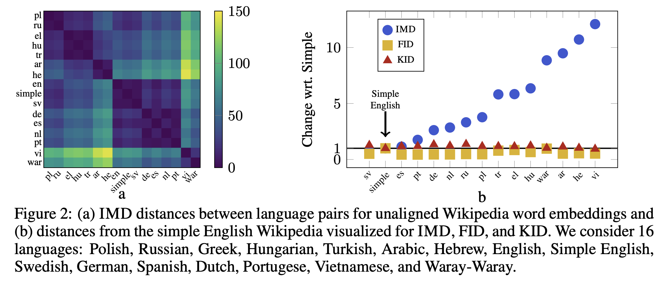
Distances between languages (original paper)
SVD and algorithms for its computations: divide-and-conquer, QR, Jacobi, bisection.
Today, we will do a brief dive into the randomized NLA.
A good read is (https://arxiv.org/pdf/2002.01387.pdf)
All the computations that we considered up to today were deterministic.
However, reduction of complexity can be done by using randomized (stochastic) computation.
Example: randomized matrix multiplication.
Checks by multiplying by random vectors!
Complexity is $k n^2$, probability is of failure is $\frac{1}{2^k}$.
But can we multiply matrices faster using randomization ideas?
Q: how to sample them?
A: generate probabilities from their norms!
where $A^{(i_t)}$ is a column of $A$ and $B_{(i_t)}$ is a row of $B$
import numpy as np

n = 1
p = 10000
m = 1
A = np.random.randn(n, p)
B = np.random.randn(p, m)
C = A @ A.T

def randomized_matmul(A, B, k):
    p1 = A.shape[1]
    p = np.linalg.norm(A, axis=0) * np.linalg.norm(B, axis=1)
    p = p
    p = p.ravel() / p.sum()
    n = A.shape[1]
    p = np.ones(p1)
    p = p/p.sum()
    idx = np.random.choice(np.arange(n), (k,), False, p)
    #d = 1 / np.sqrt(k * p[idx])
    d = 1.0/np.sqrt(k)#np.sqrt(p1)/np.sqrt(k*p[idx])
    A_sketched = A[:, idx]*np.sqrt(p1)/np.sqrt(k)#* d[None, :]
    B_sketched = B[idx, :]*np.sqrt(p1)/np.sqrt(k) #* d[:, None]
    C = A_sketched @ B_sketched
    print(d)
    return C

def randomized_matmul_topk(A, B, K):

    norm_mult = np.linalg.norm(A,axis=0) * np.linalg.norm(B,axis=1)
    top_k_idx = np.sort(np.argsort(norm_mult)[::-1][:K])

    A_top_k_cols = A[:, top_k_idx]
    B_top_k_rows = B[top_k_idx, :]

    C_approx = A_top_k_cols @ B_top_k_rows
    return C_approx

num_items = 3000
C_appr_samples = randomized_matmul(A, B, num_items)
print(C_appr_samples, 'appr')
print(C, 'true')
C_appr_topk = randomized_matmul_topk(A, B, num_items)
print(np.linalg.norm(C_appr_topk - C, 2) / np.linalg.norm(C, 2))
print(np.linalg.norm(C_appr_samples - C, 2) / np.linalg.norm(C, 2))
0.018257418583505537
[[-209.68265641]] appr
[[10065.73675927]] true
1.012091041179466
1.020831327246555
Use approximation $$ AB \approx ASD(SD)^\top B = ACC^{\top}B$$ can replace sampling and scaling with another matrix that
Q: what matrices can be used?
Many problems can be written in the form of the trace estimation:
$$\mathrm{Tr}(A) = \sum_{i} A_{ii}.$$Can we compute the trace of the matrix if we only have access to matrix-by-vector products?
The randomized trace estimators can be computed from the following formula:
$$\mathrm{Tr}(A) = E_w w^* A w, \quad E ww^* = 1$$In order to sample, we pick $k$ independent samples of $w_k$, get random variable $X_k$ and average the results.
Girard trace estimator: Sample $w \sim N(0, 1)$
Then, $\mathrm{Var} X_k = \frac{2}{k} \sum_{i, j=1}^n \vert A_{ij} \vert^2 = \frac{2}{k} \Vert A \Vert^2_F$
Hutchinson trace estimator: Let $w$ be a Rademacher random vector (i.e., elements are sampled from the uniform distribution.
It gives the minimal variance estimator.
The variance of the trace can be estimated in terms of intrinsic dimension (intdim) for symmetric positive definite matrices.
It is defined as $\mathrm{intdim}(A) = \frac{\mathrm{Tr}(A)}{\Vert A \Vert_F}$. It is easy to show that
$$1 \leq \mathrm{intdim}(A) \leq r.$$Then, the probability of the large deviation can be estimated as
$$P( \vert \overline{X}_k - \mathrm{Tr}(A) \vert \geq t \mathrm{Tr}(A)) \leq \frac{2}{k \mathrm{intdim}(A) t^2}$$If $A$ is SPD, then
$$P(\overline{X}_k \geq \tau \mathrm{Tr}(A) ) \leq \exp\left(-1/2 \mathrm{intdim}(A) (\sqrt{\tau} - 1)^2)\right) $$Similar inequality holds for the lower bound.
This estimate is much better.
An interesting (and often mislooked) property of stochastic estimator is that it comes with a stochastic variance estimate (from samples!)
Warning: we still need $\varepsilon^{-2}$ samples to get to the accuracy $\varepsilon$ when using independent samples.
where $A$ is of size $m \times n$, $U$ is of size $m \times k$ and $V$ is of size $n \times k$.
Then the following deterministic steps can give the factors $U$, $\Sigma$ and $V$ corresponding of SVD of matrix $A$
If $k \ll \min(m, n)$ then these steps can be performed fast
import matplotlib.pyplot as plt
import numpy as np

n = 1000
k = 100
m = 200
# Lowrank matrix
A = np.random.randn(n, k)
B = np.random.randn(k, m)
A = A @ B

# Random matrix
# A = np.random.randn(n, m)

def randomized_svd(A, rank, p):
    m, n = A.shape
    G = np.random.randn(n, rank + p)
    Y = A @ G
    Q, _ = np.linalg.qr(Y)
    B = Q.T @ A
    u, S, V = np.linalg.svd(B)
    U = Q @ u
    return U, S, V

rank = 100
p = 20
U, S, V = randomized_svd(A, rank, p)
print("Error from randomized SVD", np.linalg.norm(A - U[:, :rank] * S[None, :rank] @ V[:rank, :]))
plt.semilogy(S[:rank] / S[0], label="Random SVD")
u, s, v = np.linalg.svd(A)
print("Error from exact SVD", np.linalg.norm(A - u[:, :rank] * s[None, :rank] @ v[:rank, :]))
plt.semilogy(s[:rank] / s[0], label="Exact SVD")
plt.legend(fontsize=18)
plt.xticks(fontsize=16)
plt.yticks(fontsize=16)
plt.ylabel("$\sigma_i / \sigma_0$", fontsize=16)
_ = plt.xlabel("Index of singular value", fontsize=16)
Error from randomized SVD 1.4025109617270866e-11
Error from exact SVD 1.236565947080769e-11

import scipy.sparse.linalg as spsplin
# More details about Facebook package for computing randomized SVD is here: https://research.fb.com/blog/2014/09/fast-randomized-svd/
import fbpca
n = 1000
m = 200
A = np.random.randn(n, m)
k = 10
p = 10
%timeit spsplin.svds(A, k=k)
%timeit randomized_svd(A, k, p)
%timeit fbpca.pca(A, k=k, raw=False)
59.7 ms ± 6.14 ms per loop (mean ± std. dev. of 7 runs, 10 loops each)
18.7 ms ± 2.69 ms per loop (mean ± std. dev. of 7 runs, 10 loops each)
15.5 ms ± 2.46 ms per loop (mean ± std. dev. of 7 runs, 100 loops each)
The averaged error of the presented algorithm, where $k$ is target rank and $p$ is oversampling parameter, is the following
The expectation is taken w.r.t. random matrix $G$ generated in the method described above.
Compare these upper bounds with Eckart-Young theorem. Are these bounds good?
n = 1000
m = 200
A = np.random.randn(n, m)
s = np.linalg.svd(A, compute_uv=False)
Aq = A @ A.T @ A
sq = np.linalg.svd(Aq, compute_uv=False)
plt.semilogy(s / s[0], label="$A$")
plt.semilogy(sq / sq[0], label="$A^{(1)}$")
plt.legend(fontsize=18)
plt.xticks(fontsize=16)
plt.yticks(fontsize=16)
plt.ylabel("$\sigma_i / \sigma_0$", fontsize=16)
_ = plt.xlabel("Index of singular value", fontsize=16)

Q: how can we battle with this issue?
A: sequential orthogonalization!
def more_accurate_randomized_svd(A, rank, p, q):
    m, n = A.shape
    G = np.random.randn(n, rank + p)
    Y = A @ G
    Q, _ = np.linalg.qr(Y)
    for i in range(q):
        W = A.T @ Q
        W, _ = np.linalg.qr(W)
        Q = A @ W
        Q, _ = np.linalg.qr(Q)
    B = Q.T @ A
    u, S, V = np.linalg.svd(B)
    U = Q @ u
    return U, S, V

n = 1000
m = 200
A = np.random.randn(n, m)

rank = 100
p = 20
U, S, V = randomized_svd(A, rank, p)
print("Error from randomized SVD", np.linalg.norm(A - U[:, :rank] * S[None, :rank] @ V[:rank, :]))
plt.semilogy(S[:rank] / S[0], label="Random SVD")

Uq, Sq, Vq = more_accurate_randomized_svd(A, rank, p, 5)
print("Error from more accurate randomized SVD", np.linalg.norm(A - Uq[:, :rank] * Sq[None, :rank] @ Vq[:rank, :]))
plt.semilogy(Sq[:rank] / Sq[0], label="Accurate random SVD")

u, s, v = np.linalg.svd(A)
print("Error from exact SVD", np.linalg.norm(A - u[:, :rank] * s[None, :rank] @ v[:rank, :]))
plt.semilogy(s[:rank] / s[0], label="Exact SVD")
plt.legend(fontsize=18)
plt.xticks(fontsize=16)
plt.yticks(fontsize=16)
plt.ylabel("$\sigma_i / \sigma_0$", fontsize=16)
_ = plt.xlabel("Index of singular value", fontsize=16)
Error from randomized SVD 288.1455342798038
Error from more accurate randomized SVD 251.3959267962541
Error from exact SVD 250.50337524965528

%timeit spsplin.svds(A, k=k)
%timeit fbpca.pca(A, k=k, raw=False)
%timeit randomized_svd(A, k, p)
%timeit more_accurate_randomized_svd(A, k, p, 1)
%timeit more_accurate_randomized_svd(A, k, p, 2)
%timeit more_accurate_randomized_svd(A, k, p, 5)
58.9 ms ± 3.99 ms per loop (mean ± std. dev. of 7 runs, 10 loops each)
18.6 ms ± 1.17 ms per loop (mean ± std. dev. of 7 runs, 100 loops each)
27.9 ms ± 3.39 ms per loop (mean ± std. dev. of 7 runs, 10 loops each)
46 ms ± 6.25 ms per loop (mean ± std. dev. of 7 runs, 10 loops each)
76.2 ms ± 14.9 ms per loop (mean ± std. dev. of 7 runs, 10 loops each)
133 ms ± 19.2 ms per loop (mean ± std. dev. of 7 runs, 10 loops each)
The presented above method provides the following upper bound
$$ \mathbb{E}\|A - QQ^{\top}A \|_2 \leq \left[\left( 1 + \sqrt{\frac{k}{p-1}} \right)\sigma^{2q+1}_{k+1} + \frac{e\sqrt{k+p}}{p}\left( \sum_{j=k+1}^{\min(m, n)} \sigma^{2(2q+1)}_j \right)^{1/2}\right]^{1/(2q+1)} $$Consider the worst case, where no lowrank structure exists in the given matrix.
Q: what is the degree of suboptimality w.r.t. Eckart-Young theorem?
and given an approximation $x_k$ try to find $x_{k+1}$ as
$$x_{k+1} = \arg \min_x \frac12 \Vert x - x_k \Vert^2_2, \quad \mbox{s.t.} \quad a^{\top}_i x = f_i.$$where $\kappa_F(A) = \frac{\| A \|_F}{\sigma_{\min}(A)}$ and $\sigma_{\min}(A)$ is a minimal non-zero singular value of $A$. This result was presented in (Strohmer and Vershynin, 2009)
where $r^* = Ax^* - f$
The main idea is to use two steps of RKM:
the first step is for system $A^\top z = 0$ starting from $z_k$
$$ z^{k+1} = z^{k} - \frac{a^\top_{:, j} z^k}{\| a_{:, j} \|_2^2}a_{:, j} $$
the second step is for system $Ax = f - z_{k+1}$ starting from $x_k$
$$x^{k+1} = x^k - \frac{a_{i,:}x_k - f_i + z^{k+1}_i}{\|a_{i,:}\|_2^2}a^{\top}_{i,:} $$
Here $a_{:, j}$ denotes the $j$-th column of $A$ and $a_{i, :}$ denotes the $i$-th row of $A$
The key idea is the coherence of the matrix.
Let $A$ be $n \times r$ and $U$ be an orthogonal matrix whose columns form the basis of the column space of $A$.
Then, coherence is defined as
$$\mu(A) = \max \Vert U_{i, *} \Vert^2$$Coherence is always smaller than $1$ and bigger than $\frac{r}{n}$, it has nothing to do with the condition number.
What does it mean?
Small coherence means, that sampling rows uniformly gives a good preconditioner (will be covered later in the course, and why it is important)
One can do $S A = QR$, and look at the condition number of $AR^{-1}$.
from IPython.core.display import HTML
def css_styling():
    styles = open("./styles/custom.css", "r").read()
    return HTML(styles)
css_styling()