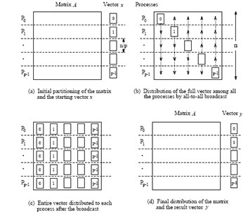
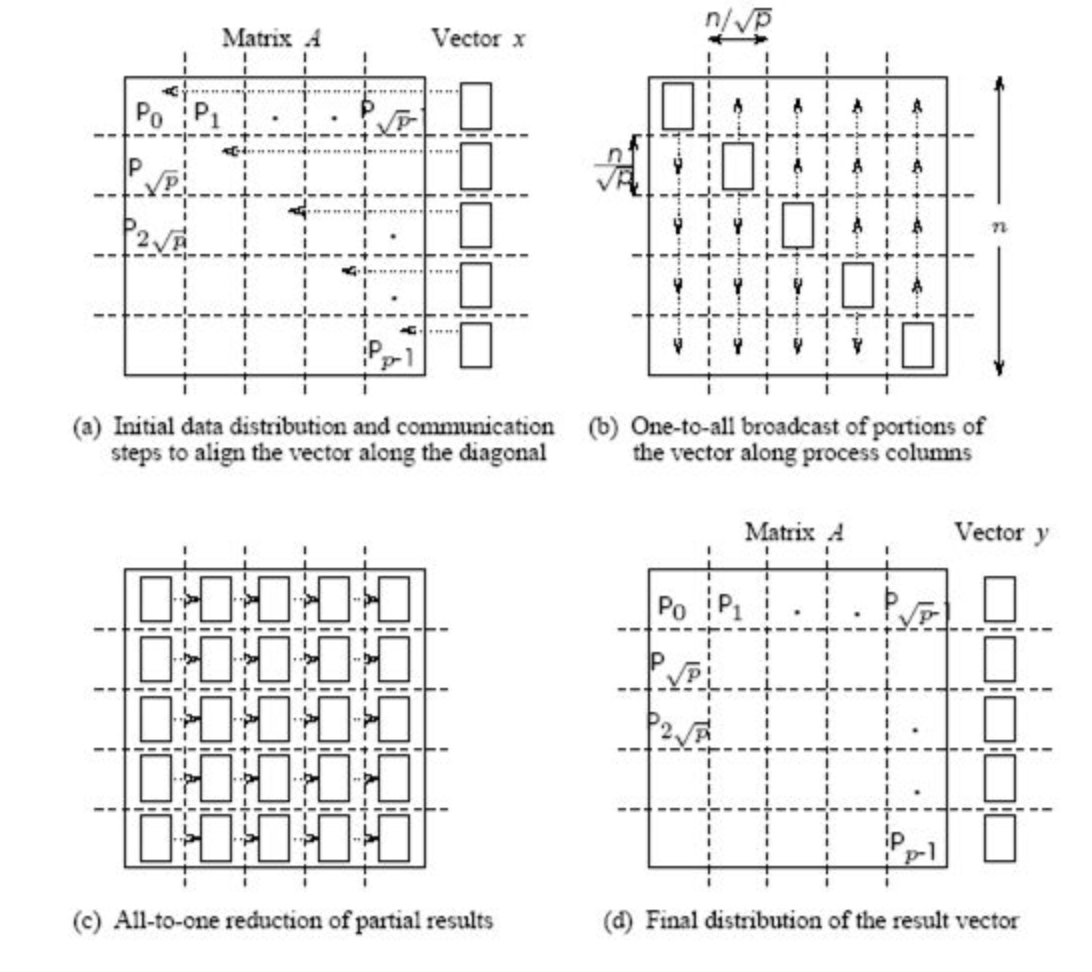
1D blocking scheme
Randomized matmul, trace, linear least squares.
For dense linear algebra problems, we are limited by the memory to store the full matrix, it is $N^2$ parameters.
The class of sparse matrices where most of the elements are zero, allows us at least to store such matrices.
The question if we can:
with sparse matrices
Now we will talk about sparse matrices, where they arise, how we store them, how we operate with them.
Sparse matrices arise in:
The simplest partial differential equation (PDE), called
Laplace equation:
$$ \Delta T = \frac{\partial^2 T}{\partial x^2} + \frac{\partial^2 T}{\partial y^2} = f(x,y), \quad x,y\in \Omega\equiv[0,1]^2, $$$$ T_{\partial\Omega} = 0. $$same for $\frac{\partial^2 T}{\partial y^2},$
and we get a linear system.
First, let us consider one-dimensional case:
After the discretization of the one-dimensional Laplace equation with Dirichlet boundary conditions we have
$$\frac{u_{i+1} + u_{i-1} - 2u_i}{h^2} = f_i,\quad i=1,\dots,N-1$$$$ u_{0} = u_N = 0$$or in the matrix form
$$ A u = f,$$and (for $n = 5$) $$A=-\frac{1}{h^2}\begin{bmatrix} 2 & -1 & 0 & 0 & 0\\ -1 & 2 & -1 & 0 &0 \\ 0 & -1 & 2& -1 & 0 \\ 0 & 0 & -1 & 2 &-1\\ 0 & 0 & 0 & -1 & 2 \end{bmatrix}$$
The matrix is triadiagonal and sparse
(and also Toeplitz: all elements on the diagonal are the same)
In two dimensions, we get equation of the form
$$-\frac{4u_{ij} -u_{(i-1)j} - u_{(i+1)j} - u_{i(j-1)}-u_{i(j+1)}}{h^2} = f_{ij},$$or in the Kronecker product form
$$\Delta_{2D} = \Delta_{1D} \otimes I + I \otimes \Delta_{1D},$$where $\Delta_{1D}$ is a 1D Laplacian, and $\otimes$ is a Kronecker product of matrices.
For matrices $A\in\mathbb{R}^{n\times m}$ and $B\in\mathbb{R}^{l\times k}$ its Kronecker product is defined as a block matrix of the form
$$ A\otimes B = \begin{bmatrix}a_{11}B & \dots & a_{1m}B \\ \vdots & \ddots & \vdots \\ a_{n1}B & \dots & a_{nm}B\end{bmatrix}\in\mathbb{R}^{nl\times mk}. $$In the block matrix form the 2D-Laplace matrix can be written in the following form:
$$A = -\frac{1}{h^2}\begin{bmatrix} \Delta_1 + 2I & -I & 0 & 0 & 0\\ -I & \Delta_1 + 2I & -I & 0 &0 \\ 0 & -I & \Delta_1 + 2I & -I & 0 \\ 0 & 0 & -I & \Delta_1 + 2I &-I\\ 0 & 0 & 0 & -I & \Delta_1 + 2I \end{bmatrix}$$More sparse matrices you can find in Florida sparse matrix collection which contains all sorts of matrices for different applications.
from IPython.display import IFrame
IFrame("http://yifanhu.net/GALLERY/GRAPHS/search.html", width=700, height=450)
We can create sparse matrix using scipy.sparse package (actually this is not the best sparse matrix package)
We can go to really large sizes (at least, to store this matrix in the memory)
Please note the following functions
spdiagskronimport numpy as np
import scipy as sp
import scipy.sparse
from scipy.sparse import csc_matrix, csr_matrix
import matplotlib.pyplot as plt
import scipy.linalg
import scipy.sparse.linalg
%matplotlib inline
n = 32
ex = np.ones(n);
lp1 = sp.sparse.spdiags(np.vstack((ex, -2*ex, ex)), [-1, 0, 1], n, n, 'csr');
e = sp.sparse.eye(n)
A = sp.sparse.kron(lp1, e) + sp.sparse.kron(e, lp1)
A = csc_matrix(A)
plt.spy(A, aspect='equal', marker='.', markersize=5)
<matplotlib.lines.Line2D at 0x10ebb9d00>

The spy command plots the sparsity pattern of the matrix: the $(i, j)$ pixel is drawn, if the corresponding matrix element is non-zero.
Sparsity pattern is really important for the understanding the complexity of the sparse linear algebra algorithms.
Often, only the sparsity pattern is needed for the analysis of "how complex" the matrix is.
The definition of "sparse matrix" is that the number of non-zero elements is much less than the total number of elements.
You can do the basic linear algebra operations (like solving linear systems at the first place) faster, than if working for with the full matrix.
Question 1: How to store the sparse matrix in memory?
Question 2: How to multiply sparse matrix by vector fast?
Question 3: How to solve linear systems with sparse matrices fast?
There are many storage formats, important ones:
In scipy there are constructors for each of these formats, e.g.
scipy.sparse.lil_matrix(A).
The simplest format is to use coordinate format to represent the sparse matrix as positions and values of non-zero elements.
i, j, val
where i, j are integer array of indices, val is the real array of matrix elements.
So we need to store $3\cdot$ nnz elements, where nnz denotes number of nonzeroes in the matrix.
Q: What is good and what is bad in this format?
First two disadvantages are solved by compressed sparse row (CSR) format.
In the CSR format a matrix is stored as 3 different arrays:
ia, ja, sa
where:
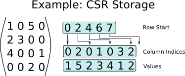
So, we got $2\cdot{\bf nnz} + n+1$ elements.
for i in range(n):

        for k in range(ia[i]:ia[i+1]):

            y[i] += sa[k] * x[ja[k]]
Let us do a short timing test
import numpy as np
import scipy as sp
import scipy.sparse
import scipy.sparse.linalg
from scipy.sparse import csc_matrix, csr_matrix, coo_matrix
import matplotlib.pyplot as plt
%matplotlib inline
n = 512
ex = np.ones(n);
lp1 = sp.sparse.spdiags(np.vstack((ex,  -2*ex, ex)), [-1, 0, 1], n, n, 'csr');
e = sp.sparse.eye(n)
A = sp.sparse.kron(lp1, e) + sp.sparse.kron(e, lp1)
A = csr_matrix(A)
rhs = np.ones(n * n)
B = coo_matrix(A)
%timeit A.dot(rhs)
%timeit B.dot(rhs)
785 µs ± 18.2 µs per loop (mean ± std. dev. of 7 runs, 1,000 loops each)
4.62 ms ± 7.62 µs per loop (mean ± std. dev. of 7 runs, 100 loops each)
As you see, CSR is faster, and for more unstructured patterns the gain will be larger.
The standard way to measure the efficiency of linear algebra operations on a particular computing architecture is to use flops (number of floating point operations per second)
We can measure peak efficiency of an ordinary matrix-by-vector product.
import numpy as np
import time
n = 4000
k = 50
a = np.random.randn(n, n)
v = np.random.randn(n, k)
t = time.time()
np.dot(a, v)
t = time.time() - t
print('Time: {0: 3.1e}, Efficiency: {1: 3.1e} Gflops'.\
      format(t,  ((k*2 * n ** 2)/t) / 10 ** 9))
Time: 2.6e-02, Efficiency: 6.2e+01 Gflops
n = 4000
k = 50
ex = np.ones(n)
a = sp.sparse.spdiags(np.vstack((ex,  -2*ex, ex)), [-1, 0, 1], n, n, 'csr');
rhs = np.random.randn(n, k)
t = time.time()
a.dot(rhs)
t = time.time() - t
print('Time: {0: 3.1e}, Efficiency: {1: 3.1e} Gflops'.\
      format(t,  (3 * n * k) / t / 10 ** 9))
Time: 4.0e-04, Efficiency: 1.5e+00 Gflops
Q: what if cache does not have free space?

for i in range(n):

        for k in range(ia[i]:ia[i+1]):

            y[i] += sa[k] * x[ja[k]]
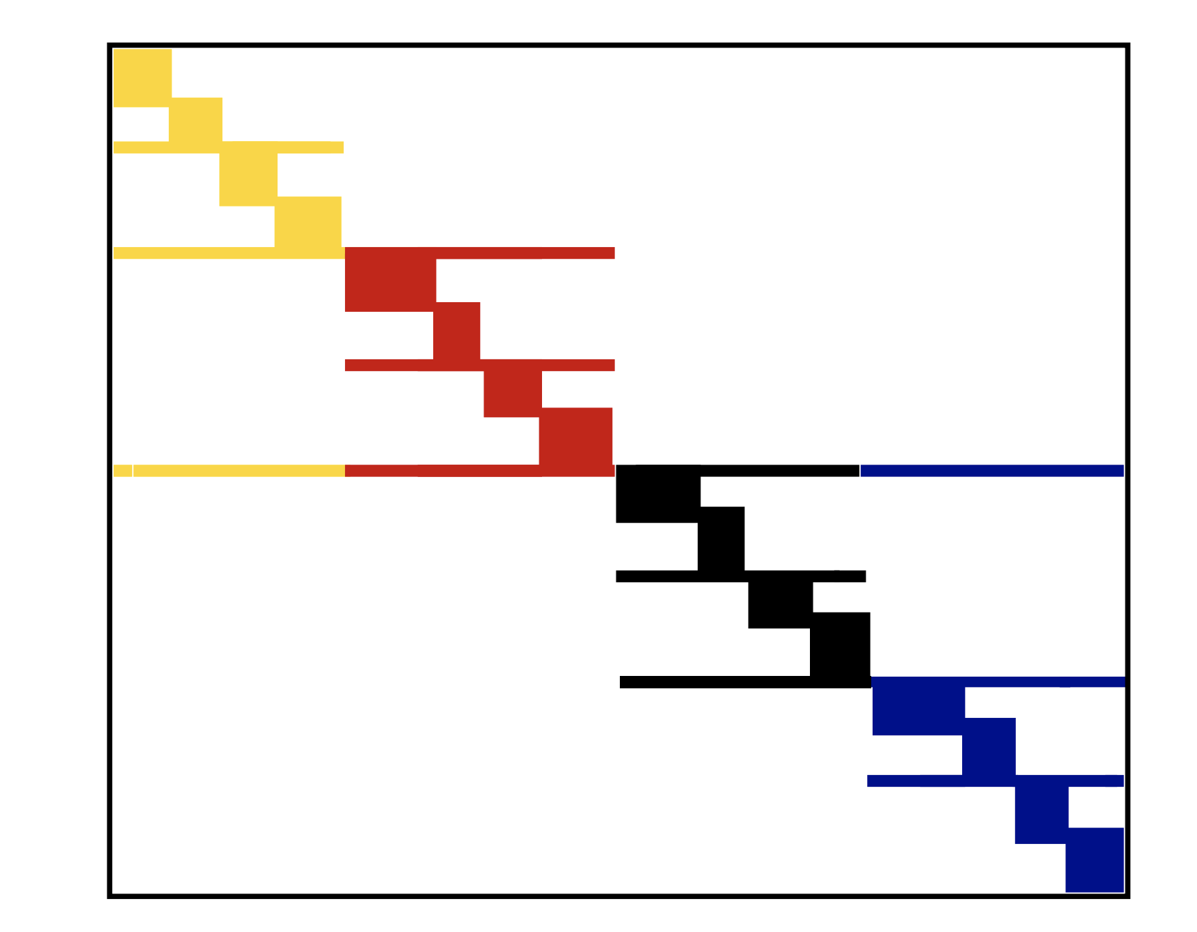
ja stores sequential elements, then they will be moved to cache altogether and number of cache misses decreasesWe can convert given sparse matrix to banded or block diagonal with permutations
Let $P$ be row permutation matrix and $Q$ be column permutation matrix
Let us start with small demo of solving sparse linear system...
n = 1024
ex = np.ones(n);
lp1 = sp.sparse.spdiags(np.vstack((ex,  -2*ex, ex)), [-1, 0, 1], n, n, 'csr');
e = sp.sparse.eye(n)
A = sp.sparse.kron(lp1, e) + sp.sparse.kron(e, lp1)
A = csr_matrix(A)
rhs = np.ones(n * n)
sol = sp.sparse.linalg.spsolve(A, rhs)
_, (ax1, ax2) = plt.subplots(1, 2)
ax1.plot(sol)
ax1.set_title('Not reshaped solution')
ax2.contourf(sol.reshape((n, n), order='f'))
ax2.set_title('Reshaped solution')
Text(0.5, 1.0, 'Reshaped solution')

from IPython.core.display import HTML
def css_styling():
    styles = open("./styles/custom.css", "r").read()
    return HTML(styles)
css_styling()