Lecture 4: Matrix rank, low-rank approximation, SVD

Previous lecture

• Peak performance of algorithm
• Complexity of matrix multiplication algorithms
• Idea of blocking (why it is good?)

Todays lecture

• Matrix rank
• Skeleton decomposition
• Low-rank approximation
• Singular Value Decomposition (SVD)
• Applications of SVD

Matrix and linear spaces

• A matrix can be considered as a sequence of vectors that are columns of a matrix:

$$ A = [a_1, \ldots, a_m], $$

where $a_m \in \mathbb{C}^{n\times 1}$.

• A matrix-by-vector product is equivalent to taking a linear combination of those columns

$$ y = Ax \quad \Longleftrightarrow \quad y = a_1 x_1 + a_2 x_2 + \ldots +a_m x_m. $$

• This is a special case of block matrix notation (columns are also blocks) that we have already seen (blocking to fit cache memory, Strassen algorithm).

Linear dependence

Definition. Vectors $a_i$ are called linearly dependent, if there exist simultaneously non-zero coefficients $x_i$ such that

$$\sum_i a_i x_i = 0,$$

or in the matrix form

$$ Ax = 0, \quad \Vert x \Vert \ne 0. $$

In this case, we say that the matrix $A$ has a non-trivial nullspace (or kernel) denoted by $N(A)$ (or $\text{ker}(A)$).

Vectors that are not linearly dependent are called linearly independent.

Linear (vector) space

A linear space spanned by vectors $\{a_1, \ldots, a_m\}$ is defined as all possible vectors of the form

$$ \mathcal{L}(a_1, \ldots, a_m) = \left\{y: y = \sum_{i=1}^m a_i x_i, \, \forall x_i, \, i=1,\dots, n \right\}, $$

In the matrix form, the linear space is a set of all $y$ such that

$$y = A x.$$

This set is also called the range (or image) of the matrix, denoted by $\text{range}(A)$ (or $\text{im}(A)$) respectively.

Dimension of a linear space

• The dimension of a linear space $\text{im}(A)$ denoted by $\text{dim}\, \text{im} (A)$ is the minimal number of vectors required to represent each vector from $\text{im} (A)$.

• The dimension of $\text{im}(A)$ has a direct connection to the matrix rank.

Matrix rank

• Rank of a matrix $A$ is a maximal number of linearly independent columns in a matrix $A$, or the dimension of its column space $= \text{dim} \, \text{im}(A)$.

• You can also use linear combination of rows to define the rank, i.e. formally there are two ranks: column rank and row rank of a matrix.

Theorem
The dimension of the column space of the matrix is equal to the dimension of its row space.

Proof

• In the matrix form this fact can be written as $\mathrm{dim}\ \mathrm{im} (A) = \mathrm{dim}\ \mathrm{im} (A^\top)$.

• Thus, there is a single rank!

Full-rank matrix

• A matrix $A \in \mathbb{R}^{m \times n}$ is called of full-rank, if $\mathrm{rank}(A) = \min(m, n)$.

Suppose, we have a linear space, spanned by $n$ vectors. Let these vectors be random with elements from standard normal distribution $\mathcal{N}(0, 1)$.

Q: What is the probability of the fact that this subspace has dimension $m < n$?

A: Random matrix has full rank with probability 1.

Dimensionality reduction

• A lot of data from real-world applications are high dimensional, for instance images (e.g. $512\times 512$ pixels), texts, graphs.
• However, working with high-dimensional data is not an easy task.
• Is it possible to reduce the dimensionality, preserving important relations between objects such as distance?

Johnson–Lindenstrauss lemma

Let $N\gg 1$. Given $0 < \epsilon < 1$, a set of $m$ points in $\mathbb{R}^N$ and $n > \frac{8 \log m}{\epsilon^2}$ (we want $n\ll N$).

Then there exists linear map $f$ from $\mathbb{R}^N \rightarrow \mathbb{R}^n$ such that the following inequality holds:

$$(1 - \epsilon) \Vert u - v \Vert^2 \leq \Vert f(u) - f(v) \Vert^2 \leq (1 + \epsilon) \Vert u - v \Vert^2.$$

• This theorem states that there exists a map from high- to a low-dimensional space so that distances between points in these spaces are almost the same.
• It is not very practical due to the dependence on $\epsilon$.
• This lemma does not give a recipe how to construct $f$, but guarantees that $f$ exists.

Skeleton decomposition

A very useful representation for computation of the matrix rank is the skeleton decomposition and is closely related to the rank. This decompositions explains, why and how matrices of low rank can be compressed.

It can be graphically represented as follows:
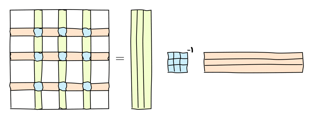or in the matrix form

$$ A = C \widehat{A}^{-1} R, $$

where $C$ are some $k=\mathrm{rank}(A)$ columns of $A$, $R$ are some $k$ rows of $A$ and $\widehat{A}$ is the nonsingular submatrix on the intersection.

Remark

We have not yet formally defined the inverse, so just a reminder:

• An inverse of the matrix $P$ is the matrix $Q = P^{-1}$ such that $ P Q = QP = I$.
• If the matrix is square and has full rank then the inverse exists.

Proof for the skeleton decomposition

• Let $C\in \mathbb{C}^{n\times k}$ be the $k$ columns based on the nonsingular submatrix $\widehat{A}$. Therefore they are linearly independent.

• Take any other column $a_i$ of $A$. Then $a_i$ can be represented as a linear combination of the columns of $C$, i.e. $a_i = C x_i$, where $x_i$ is a vector of coefficients.

• $a_i = C x_i$ are $n$ equations. We take $k$ equations of those corresponding to the rows that contain $\widehat{A}$ and get the equation

$$\widehat{r}_i = \widehat{A} x_i \quad \Longrightarrow \quad x_i = \widehat{A}^{-1} \widehat r_i$$

Thus, $a_i = C\widehat{A}^{-1} \widehat r_i$ for every $i$ and

$$A = [a_1,\dots, a_m] = C\widehat{A}^{-1} R.$$

A closer look on the skeleton decomposition

• Any rank-$r$ matrix can be written in the form

$$A = C \widehat{A}^{-1} R,$$

where $C$ is $n \times r$, $R$ is $r \times m$ and $\widehat{A}$ is $r \times r$, or

$$ A = UV, $$

where $U$ and $V$ are not unique, e.g. $U = C \widehat{A}^{-1}$, $V=R$.

• The form $A = U V$ is standard for skeleton decomposition.

• Thus, every rank-$r$ matrix can be written as a product of a "skinny" ("tall") matrix $U$ by a "fat" ("short") matrix $V$.

In the index form, it is

$$ a_{ij} = \sum_{\alpha=1}^r u_{i \alpha} v_{\alpha j}. $$

For rank 1, we have

$$ a_{ij} = u_i v_j, $$

i.e. it is a separation of indices and rank-$r$ is a sum of rank-$1$ matrices!

Storage

It is interesting to note, that for the rank-$r$ matrix

$$A = U V$$

only $U$ and $V$ can be stored, which gives us $(n+m) r$ parameters, so it can be used for compression. We can also compute matrix-by-vector $Ax$ product much faster:

• Multiplication $y = Vx$ costs $\mathcal{O}(mr)$ flops.
• Multiplication $z = Uy$ costs $\mathcal{O}(nr)$ flops.

The same works for addition, elementwise multiplication, etc. For addition:

$$ A_1 + A_2 = U_1 V_1 + U_2 V_2 = [U_1|U_2] [V_1^\top|V_2^\top]^\top $$

#A fast matrix-by-vector product demo
import jax
import jax.numpy as jnp
n = 10000
r = 10
u = jax.random.normal(jax.random.PRNGKey(0), (n, r))
v = jax.random.normal(jax.random.PRNGKey(10), (n, r))
a = u @ v.T
x = jax.random.normal(jax.random.PRNGKey(1), (n,))
print(n*n/(2*n*r))
%timeit (a @ x).block_until_ready()
%timeit (u @ (v.T @ x)).block_until_ready()

500.0
8.64 ms ± 97.4 µs per loop (mean ± std. dev. of 7 runs, 100 loops each)
97.4 µs ± 1.16 µs per loop (mean ± std. dev. of 7 runs, 10,000 loops each)

Computing matrix rank

We can also try to compute the matrix rank using the built-in jnp.linalg.matrix_rank function

#Computing matrix rank
import jax.numpy as jnp
n = 50 
a = jnp.ones((n, n))
print('Rank of the matrix:', jnp.linalg.matrix_rank(a))
b = a + 1e-8 * jax.random.normal(jax.random.PRNGKey(10), (n, n))
print('Rank of the matrix:', jnp.linalg.matrix_rank(b, tol=1e-8))

Rank of the matrix: 1
Rank of the matrix: 6

So, small perturbations might crucially affect the rank!

Instability of the matrix rank

For any rank-$r$ matrix $A$ with $r < \min(m, n)$ there is a matrix $B$ such that its rank is equal to $\min(m, n)$ and

$$ \Vert A - B \Vert = \epsilon. $$

Q: So, does this mean that numerically matrix rank has no meaning? (I.e., small perturbations lead to full rank!)

A: No. We should find a matrix $B$ such that $\|A-B\| = \epsilon$ and $B$ has minimal rank. So we can only compute rank with given accuracy $\epsilon$. One of the approaches to compute matrix rank $r$ is SVD.

Low rank approximation

The important problem in many applications is to find low-rank approximation of the given matrix with given accurcacy $\epsilon$ or rank $r$.
Examples:

• principal component analysis
• recommender systems
• least squares
• neural network compression

These problems can be solved by SVD.

Singular value decomposition

To compute low-rank approximation, we need to compute singular value decomposition (SVD).

Theorem Any matrix $A\in \mathbb{C}^{n\times m}$ can be written as a product of three matrices:

$$ A = U \Sigma V^*, $$

where

• $U$ is an $n \times K$ unitary matrix,
• $V$ is an $m \times K$ unitary matrix, $K = \min(m, n)$,
• $\Sigma$ is a diagonal matrix with non-negative elements $\sigma_1 \geq \ldots, \geq \sigma_K$ on the diagonal.
• Moreover, if $\text{rank}(A) = r$, then $\sigma_{r+1} = \dots = \sigma_K = 0$.

Proof

• Matrix $A^*A$ is Hermitian, hence diagonalizable in unitary basis (will be discussed further in the course).
• $A^*A\geq0$ (non-negative definite), so eigenvalues are non-negative. Therefore, there exists unitary matrix $V = [v_1, \dots, v_n]$ such that

$$ V^* A^* A V = \text{diag}(\sigma_1^2,\dots, \sigma_n^2), \quad \sigma_1\geq \sigma_2\geq \dots \geq \sigma_n. $$

Let $\sigma_i = 0$ for $i>r$, where $r$ is some integer.
Let $V_r= [v_1, \dots, v_r]$, $\Sigma_r = \text{diag}(\sigma_1, \dots,\sigma_r)$. Hence

$$ V^*_r A^* A V_r = \Sigma_r^2 \quad \Longrightarrow \quad (\Sigma_r^{-1} V_r^* A^*) (A V_r\Sigma_r^{-1} ) = I. $$

As a result, matrix $U_r = A V_r\Sigma_r^{-1}$ satisfies $U_r^* U_r = I$ and hence has orthogonal columns.
Let us add to $U_r$ any orthogonal columns that are orthogonal to columns in $U_r$ and denote this matrix as $U$. Then

$$ AV = U \begin{bmatrix} \Sigma_r & 0 \\ 0 & 0 \end{bmatrix}\quad \Longrightarrow \quad U^* A V = \begin{bmatrix}\Sigma_r & 0 \\ 0 & 0 \end{bmatrix}. $$

Since multiplication by non-singular matrices does not change rank of $A$, we have $r = \text{rank}(A)$.

Corollary 1: $A = \displaystyle{\sum_{\alpha=1}^r} \sigma_\alpha u_\alpha v_\alpha^*$ or elementwise $a_{ij} = \displaystyle{\sum_{\alpha=1}^r} \sigma_\alpha u_{i\alpha} \overline{v}_{j\alpha}$

Corollary 2: $$\text{ker}(A) = \mathcal{L}\{v_{r+1},\dots,v_n\}$$

$$\text{im}(A) = \mathcal{L}\{u_{1},\dots,u_r\}$$$$\text{ker}(A^*) = \mathcal{L}\{u_{r+1},\dots,u_n\}$$$$\text{im}(A^*) = \mathcal{L}\{v_{1},\dots,v_r\}$$

Eckart-Young theorem

The best low-rank approximation can be computed by SVD.

Theorem: Let $r < \text{rank}(A)$, $A_r = U_r \Sigma_r V_r^*$. Then

$$ \min_{\text{rank}(B)=r} \|A - B\|_2 = \|A - A_r\|_2 = \sigma_{r+1}. $$

The same holds for $\|\cdot\|_F$, but $\|A - A_r\|_F = \sqrt{\sigma_{r+1}^2 + \dots + \sigma_{\min (n,m)}^2}$.

Proof

• Since $\text{rank} (B) = r$, it holds $\text{dim}~\text{ker}~B = n-r$.
• Hence there exists $z\not=0$ such that $z\in \text{ker}(B) \cap \mathcal{L}(v_1,\dots,v_{r+1})$ (as $\text{dim}\{v_1,\dots,v_{r+1}\} = r+1$).
• Fix $\|z\| = 1$. Therefore,

$$ \|A-B\|_2^2 \geq \|(A-B)z\|_2^2 = \|Az\|_2^2 = \| U\Sigma V^* z\|^2_2= \|\Sigma V^* z\|^2_2 = \sum_{i=1}^{n} \sigma_i^2 (v_i^*z)^2 =\sum_{i=1}^{r+1} \sigma_i^2 (v_i^*z)^2 \geq \sigma_{r+1}^2\sum_{i=1}^{r+1} (v_i^*z)^2 = \sigma_{r+1}^2 $$

as $\sigma_1\geq \dots \geq \sigma_{r+1}$ and $$\sum_{i=1}^{r+1} (v_i^*z)^2 = \|V^*z\|_2^2 = \|z\|_2^2 = 1.$$

Main result on low-rank approximation

Corollary: computation of the best rank-$r$ approximation is equivalent to setting $\sigma_{r+1}= 0, \ldots, \sigma_K = 0$. The error

$$ \min_{A_r} \Vert A - A_r \Vert_2 = \sigma_{r+1}, \quad \min_{A_r} \Vert A - A_r \Vert_F = \sqrt{\sigma_{r+1}^2 + \dots + \sigma_{K}^2} $$

that is why it is important to look at the decay of the singular values.

Computing SVD

• Algorithms for the computation of the SVD are tricky and will be discussed later.

• But for numerics, we can use NumPy or JAX or PyTorch already!

Let us go back to the previous example

#Computing matrix rank
import jax.numpy as jnp
n = 50 
a = jnp.ones((n, n))
print('Rank of the matrix:', jnp.linalg.matrix_rank(a))
b = a + 1e-5 * jax.random.normal(jax.random.PRNGKey(-1), (n, n))
print('Rank of the matrix:', jnp.linalg.matrix_rank(b, tol=1e-3))

Rank of the matrix: 1
Rank of the matrix: 1

u, s, v = jnp.linalg.svd(b) #b = u@jnp.diag(s)@v 
print(s/s[0])
print(s[1]/s[0])
r = 1
u1 = u[:, :r]
s1 = s[:r]
v1 = v[:r, :]
a1 = u1.dot(jnp.diag(s1).dot(v1))
print(jnp.linalg.norm(b - a1, 2)/s[0])

[1.0000000e+00 2.6038917e-06 2.5778331e-06 2.4328988e-06 2.3946168e-06
 2.3161633e-06 2.1771170e-06 2.1350679e-06 2.0692341e-06 1.9072305e-06
 1.8897628e-06 1.7940382e-06 1.7782966e-06 1.7084487e-06 1.6727121e-06
 1.6017437e-06 1.5731581e-06 1.4549468e-06 1.4165987e-06 1.3679330e-06
 1.3424550e-06 1.2941907e-06 1.2687507e-06 1.2097146e-06 1.1957062e-06
 1.1181866e-06 1.1178938e-06 1.0891903e-06 1.0027645e-06 9.4870353e-07
 8.8112211e-07 8.7050188e-07 8.0722310e-07 7.6571308e-07 6.4515058e-07
 6.0674591e-07 5.7988444e-07 4.8432429e-07 4.7683716e-07 4.7153273e-07
 4.2522197e-07 3.7936982e-07 3.2457302e-07 2.7898491e-07 2.7062282e-07
 2.3026750e-07 1.8749994e-07 1.4638464e-07 1.2981367e-07 1.7708503e-08]
2.6038917e-06
2.6034543e-06

Separation of variables for 2D functions

We can use SVD to compute approximations of function-related matrices, i.e. the matrices of the form

$$a_{ij} = f(x_i, y_j),$$

where $f$ is a certain function, and $x_i, \quad i = 1, \ldots, n$ and $y_j, \quad j = 1, \ldots, m$ are some one-dimensional grids.

%matplotlib inline
import numpy as np
import matplotlib.pyplot as plt
plt.rc("text", usetex=True)

n = 100
a = [[1.0/(i+j+1) for i in range(n)] for j in range(n)] #Hilbert matrix 
#a = jnp.ones((n, n)) + 1e-3*jax.random.normal(jax.random.PRNGKey(67575), (n, n))
a = jnp.array(a)
u, s, v = jnp.linalg.svd(a)
plt.semilogy(s[:30]/s[0], 'x')
plt.ylabel(r"$\sigma_i / \sigma_0$", fontsize=24)
plt.xlabel(r"Singular value index, $i$", fontsize=24)
plt.grid(True)
plt.xticks(fontsize=26)
plt.yticks(fontsize=26)
#We have very good low-rank approximation of it!

(array([1.e-09, 1.e-08, 1.e-07, 1.e-06, 1.e-05, 1.e-04, 1.e-03, 1.e-02,
        1.e-01, 1.e+00, 1.e+01, 1.e+02]),
 [Text(0, 1e-09, '$\\mathdefault{10^{-9}}$'),
  Text(0, 1e-08, '$\\mathdefault{10^{-8}}$'),
  Text(0, 1e-07, '$\\mathdefault{10^{-7}}$'),
  Text(0, 1e-06, '$\\mathdefault{10^{-6}}$'),
  Text(0, 1e-05, '$\\mathdefault{10^{-5}}$'),
  Text(0, 0.0001, '$\\mathdefault{10^{-4}}$'),
  Text(0, 0.001, '$\\mathdefault{10^{-3}}$'),
  Text(0, 0.01, '$\\mathdefault{10^{-2}}$'),
  Text(0, 0.1, '$\\mathdefault{10^{-1}}$'),
  Text(0, 1.0, '$\\mathdefault{10^{0}}$'),
  Text(0, 10.0, '$\\mathdefault{10^{1}}$'),
  Text(0, 100.0, '$\\mathdefault{10^{2}}$')])

Function approximation

import jax.numpy as jnp
n = 128
t = jnp.linspace(0, 5, n)
x, y = jnp.meshgrid(t, t)
f = 1.0 / (x + y + 0.01) # test your own function. Check 1.0 / (x - y + 0.5)
u, s, v = jnp.linalg.svd(f, full_matrices=False)
r = 10
u = u[:, :r]
s = s[:r]
v = v[:r, :] # Mind the transpose here!
fappr = (u * s[None, :]) @ v
er = jnp.linalg.norm(fappr - f, 'fro') / jnp.linalg.norm(f, 'fro')
print(er)
plt.semilogy(s/s[0])
plt.ylabel(r"$\sigma_i / \sigma_0$", fontsize=24)
plt.xlabel(r"Singular value index, $i$", fontsize=24)
plt.grid(True)
plt.xticks(fontsize=26)
plt.yticks(fontsize=26)

2.604117e-07

(array([1.e-08, 1.e-07, 1.e-06, 1.e-05, 1.e-04, 1.e-03, 1.e-02, 1.e-01,
        1.e+00, 1.e+01, 1.e+02]),
 [Text(0, 1e-08, '$\\mathdefault{10^{-8}}$'),
  Text(0, 1e-07, '$\\mathdefault{10^{-7}}$'),
  Text(0, 1e-06, '$\\mathdefault{10^{-6}}$'),
  Text(0, 1e-05, '$\\mathdefault{10^{-5}}$'),
  Text(0, 0.0001, '$\\mathdefault{10^{-4}}$'),
  Text(0, 0.001, '$\\mathdefault{10^{-3}}$'),
  Text(0, 0.01, '$\\mathdefault{10^{-2}}$'),
  Text(0, 0.1, '$\\mathdefault{10^{-1}}$'),
  Text(0, 1.0, '$\\mathdefault{10^{0}}$'),
  Text(0, 10.0, '$\\mathdefault{10^{1}}$'),
  Text(0, 100.0, '$\\mathdefault{10^{2}}$')])

And 3d plots...

%matplotlib inline
import matplotlib.pyplot as plt
from mpl_toolkits.mplot3d import Axes3D
# plt.xkcd()
fig = plt.figure(figsize=(10, 5))
ax = fig.add_subplot(121, projection='3d')
ax.plot_surface(x, y, f)
ax.set_title('Original function')
ax = fig.add_subplot(122, projection='3d')
ax.plot_surface(x, y, fappr - f)
ax.set_title('Approximation error with rank=%d, err=%3.1e' % (r, er))
fig.subplots_adjust()
fig.tight_layout()

Singular values of a random Gaussian matrix

What is the singular value decay of a random matrix?

import numpy as np
import matplotlib.pyplot as plt
n = 1000
a = jax.random.normal(jax.random.PRNGKey(244747), (n, n))
u, s, v = jnp.linalg.svd(a)
plt.semilogy(s/s[0])
plt.ylabel(r"$\sigma_i / \sigma_0$", fontsize=24)
plt.xlabel(r"Singular value index, $i$", fontsize=24)
plt.grid(True)
plt.xticks(fontsize=26)
plt.yticks(fontsize=26)

(array([1.e-06, 1.e-05, 1.e-04, 1.e-03, 1.e-02, 1.e-01, 1.e+00, 1.e+01,
        1.e+02]),
 [Text(0, 1e-06, '$\\mathdefault{10^{-6}}$'),
  Text(0, 1e-05, '$\\mathdefault{10^{-5}}$'),
  Text(0, 0.0001, '$\\mathdefault{10^{-4}}$'),
  Text(0, 0.001, '$\\mathdefault{10^{-3}}$'),
  Text(0, 0.01, '$\\mathdefault{10^{-2}}$'),
  Text(0, 0.1, '$\\mathdefault{10^{-1}}$'),
  Text(0, 1.0, '$\\mathdefault{10^{0}}$'),
  Text(0, 10.0, '$\\mathdefault{10^{1}}$'),
  Text(0, 100.0, '$\\mathdefault{10^{2}}$')])

Linear factor analysis & low-rank

Consider a linear factor model,

$$y = Ax, $$

where $y$ is a vector of length $n$, and $x$ is a vector of length $r$.
The data is organized as samples: we observe vectors

$$y_1, \ldots, y_T,$$

but do not know matrix $A$, then the factor model can be written as

$$ Y = AX, $$

where $Y$ is $n \times T$, $A$ is $n \times r$ and $X$ is $r \times T$.

• This is exactly a rank-$r$ model: it tells us that the vectors lie in a small subspace.
• We also can use SVD to recover this subspace (but not the independent components).
• Principal component analysis can be done by SVD, checkout the implementation in sklearn package.

Applications of SVD

• SVD is extremely important in computational science and engineering.

• It has many names: Principal component analysis, Proper Orthogonal Decomposition, Empirical Orthogonal Functions

• Now we will consider compression of dense matrix and active subspaces method

Dense matrix compression

Dense matrices typically require $N^2$ elements to be stored. A rank-$r$ approximation can reduces this number to $\mathcal{O}(Nr)$

import numpy as np
%matplotlib inline
import matplotlib.pyplot as plt

n = 256
a = [[1.0/(i - j + 0.5) for i in range(n)] for j in range(n)]
a = np.array(a)
#u, s, v = np.linalg.svd(a)
u, s, v = jnp.linalg.svd(a[n//2:, :n//2])
plt.semilogy(s/s[0])
plt.ylabel(r"$\sigma_i / \sigma_0$", fontsize=24)
plt.xlabel(r"Singular value index, $i$", fontsize=24)
plt.grid(True)
plt.xticks(fontsize=26)
plt.yticks(fontsize=26)
#s[0] - jnp.pi
#u, s, v = jnp.linalg.svd(a[:128:, :128])
#print(s[0]-jnp.pi)

DeviceArray(-0.3372376, dtype=float32)

Compression of parameters in fully-connected neural networs

• One of the main building blocks of the modern deep neural networks is fully-connected layer a.k.a. linear layer
• This layer implements the action of a linear function to an input vector: $f(x) = Wx + b$, where $W$ is a trainable matrix and $b$ is a trainable bias vector
• Both $W$ and $b$ are updated during training of the network according to some optimization method, i.e. SGD, Adam, etc...
• However, the storing of the trained optimal parameters ($W$ and $b$) can be prohibitive if you want to port your trained network to the device, where memory is limited
• As a possible recipe, you can compress matrices $W_i$ from the $i$-th linear layer with the truncated SVD based on the singular values!
• What do you get after such apprioximation of $W$?
  • memory efficient storage
  • faster inference
  • moderate degradation of the accuracy in solving the target task, i.e. image classification

Active Subspaces

• Suppose, we are given a function $f(x), \ x \in \mathcal{X} \subseteq \mathbb{R}^{n}$ and want find its low-dimensional parametrization. Here $\mathcal{X}$ is the domain of $f(x)$.

• Informally, we are searching for the directions in which a $f(x)$ changes a lot on average and for the directions in which $f(x)$ is almost constant.

• Formally, we assume that there is a matrix $W \in \mathbb{R}^{r \times n}$ and a function $g: \mathbb{R^r} \to \mathbb{R}$, such that for every $x \in \mathcal{X}$

$$ f(x) \approx g(W x). $$

How to discover Active Subspaces:

Using SVD:

1. Choose $m$, the number of estimations. This hyperparameter stands for the number of Monte Carlo estimations. The larger $m$, the more accurate the result is.
2. Draw samples $\lbrace x_i \rbrace_{i = 1}^{m}$ from $\mathcal{X}$ (according to some prior probability density function)
3. For each $x_i$ compute $\nabla f(x_i)$
4. Compute the SVD of the matrix

$$ G := \dfrac{1}{\sqrt{m}} \begin{bmatrix} \nabla f(x_1) & \nabla f(x_2) & \ldots & \nabla f(x_m) \end{bmatrix} \approx U \Sigma V^\top. $$

1. Estimate the rank of $G \approx U_r \Sigma_r V_r^\top$. The rank $r$ of the matrix $G$ is the dimensionality of the active subspace.
2. Low-dimensional vectors are estimated as $x_{\text{AS}} = U_r^\top x$.

For further details, look into the book „Active Subspaces: Emerging Ideas in Dimension Reduction for Parameter Studies“ (2015) by Paul Constantine.

Take home message

• Matrix rank definition
• Skeleton approximation and dyadic representation of a rank-$r$ matrix
• Singular value decomposition and Eckart-Young theorem
• Three applications of SVD (linear factor analysis, dense matrix compression, active subspaces).

Next lecture

• Linear systems
• Inverse matrix
• Condition number
• Linear least squares
• Pseudoinverse

Questions?

from IPython.core.display import HTML
def css_styling():
    styles = open("../styles/custom.css", "r").read()
    return HTML(styles)
css_styling()