Lecture 6: Linear systems

Previous lecture

• Matrix rank
• Skeleton decomposition
• Low-rank approximation
• Singular Value Decomposition (SVD)

Today lecture

• Linear systems
• Inverse matrix
• Condition number
• Gaussian elimination

Linear systems

• Linear systems of equations are the basic tool in NLA.

• They appear as:

  • Linear regression problems
  • Discretization of partial differential/integral equations
  • Linearizations of nonlinear regression problems
  • Optimization (i.e., Gauss-Newton and Newton-Raphson methods, KKT)

Linear equations and matrices

• From school we know about linear equations.

• A linear system of equations can be written in the form

\begin{align*} &2 x + 3 y = 5\quad &\longrightarrow \quad &2x + 3 y + 0 z = 5\\ &2 x + 3z = 5\quad &\longrightarrow\quad &2 x + 0 y + 3 z = 5\\ &x + y = 2\quad &\longrightarrow\quad & 1 x + 1 y + 0 z = 2\\ \end{align*}

Matrix form

$$ \begin{pmatrix} 2 & 3 & 0 \\ 2 & 0 & 3 \\ 1 & 1 & 0 \\ \end{pmatrix}\begin{pmatrix} x \\ y \\ z \end{pmatrix} = \begin{pmatrix} 5 \\ 5 \\ 2 \end{pmatrix} $$

or simply

$$ A u = f, $$

where $A$ is a $3 \times 3$ matrix and $f$ is right-hand side

Over/under determined linear systems

If the system $Au = f$ has

• more equations than unknowns it is called overdetermined system (generically, no solution)

• less equations than unknowns it is called underdetermined system (solution is non-unique, to make it unique additional assumptions have to be made)

Existence of solutions

A solution to the linear system of equations with a square matrix $A$

$$A u = f$$

exists, iff

• $\det A \ne 0$

or

• matrix $A$ has full rank.

Scales of linear systems

In different applications, the typical size of the linear systems can be different.

• Small: $n \leq 10^4$ (full matrix can be stored in memory, dense matrix)
• Medium: $n = 10^4 - 10^6$ (typically, sparse or structured matrix)
• Large: $n = 10^8 - 10^9$ (typically sparse matrix + parallel computations)

Linear systems can be big

• We take a continious problem, discretize it on a mesh with $N$ elements and get a linear system with $N\times N$ matrix.
• Example of a mesh around A319 aircraft (taken from GMSH website).
  

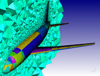
The main difficulty is that these systems are big: millions or billions of unknowns!

Linear systems can be structured

• Storing $N^2$ elements of a matrix is prohibitive even for $N = 100000$.

Q: how to work with such matrices?

A: fortunately, those matrices are structured and require $\mathcal{O}(N)$ parameters to be stored.

• The most widespread structure are sparse matrices: such matrices have only $\mathcal{O}(N)$ non-zeros!

• Example (one of the famous matrices around for $n = 5$):

$$ \begin{pmatrix} 2 & -1 & 0 & 0 & 0 \\ -1 & 2 & -1 & 0 & 0 \\ 0 & -1 & 2 & -1 & 0 \\ 0 & 0 &-1& 2 & -1 \\ 0 & 0 & 0 & -1 & 2 \\ \end{pmatrix} $$

• At least you can store such matrices
• Also you can multiply such matrix by vector fast
• But how to solve linear systems?

Main questions about linear systems

1. What is the accuracy we get from the solution (due to rounding errors)?
2. How we compute the solution? (LU-decomposition, Gaussian elimination)
3. What is the complexity of the solution of linear systems?

How to solve linear systems?

Important: forget about determinants and the Cramer rule (it is good for $2 \times 2$ matrices still)!

How to solve linear systems?

The main tool is variable elimination.

\begin{align*} &2 y + 3 x = 5 \quad&\longrightarrow \quad &y = 5/2 - 3/2 x \\ &2 x + 3z = 5 \quad&\longrightarrow\quad &z = 5/3 - 2/3 x\\ &z + y = 2 \quad&\longrightarrow\quad & 5/2 + 5/3 - (3/2 + 2/3) x = 2,\\ \end{align*}

and that is how you find $x$ (and all previous ones).

This process is called Gaussian elimination and is one of the most widely used algorithms.

Gaussian elimination

Gaussian elimination consists of two steps:

1. Forward step
2. Backward step

Forward step

• In the forward step, we eliminate $x_1$:

$$ x_1 = f_1 - (a_{12} x_2 + \ldots + a_{1n} x_n)/a_{11}, $$

and then substitute this into the equations $2, \ldots, n$.

• Then we eliminate $x_2$ and so on from the second equation.

• The important thing is that the pivots (that we divide over) are not equal to $0$.

Backward step

In the backward step:

• solve equation for $x_n$
• put it into the equation for $x_{n-1}$ and so on, until we compute all $x_i, i=1,\ldots, n$.

Gaussian elimination and LU decomposition

• Gaussian elimination is the computation of one of the most important matrix decompositions: LU-decomposition.

Definition: LU-decomposition of the square matrix $A$ is the representation

$$A = LU,$$

where

• $L$ is lower triangular (elements strictly above the diagonal are zero)
• $U$ is upper triangular matrix (elements strictly below the diagonal are zero)

This factorization is non-unique, so it is typical to require that the matrix $L$ has ones on the diagonal.

Main goal of the LU decomposition is to solve linear system, because

$$ A^{-1} f = (L U)^{-1} f = U^{-1} L^{-1} f, $$

and this reduces to the solution of two linear systems forward step

$$ L y = f, $$

and backward step

$$ U x = y. $$

Does $LU$ decomposition always exist?

Complexity of the Gaussian elimination/LU decomposition

• Each elimination step requires $\mathcal{O}(n^2)$ operations.

• Thus, the cost of the naive algorithm is $\mathcal{O}(n^3)$.

Think a little bit: can Strassen algorithm help here?

Block LU-decomposition

We can try to compute block version of LU-decomposition:

$$\begin{pmatrix} A_{11} & A_{12} \\ A_{21} & A_{22} \end{pmatrix} = \begin{pmatrix} L_{11} & 0 \\ L_{21} & L_{22} \end{pmatrix} \begin{pmatrix} U_{11} & U_{12} \\ 0 & U_{22} \end{pmatrix} $$

• There are two basic operations: compute LU-factorization of half-matrices + matrix-by-matrix product.

Existence of the LU-decomposition

• The LU-decomposition algorithm does not fail if we do not divide by zero at every step of the Gaussian elimination.

Q: when it is so, for which class of matrices?

A: it is true for strictly regular matrices.

Strictly regular matrices and LU decomposition

• Definition. A matrix $A$ is called strictly regular, if all of its leading principal minors (i.e, submatrices in the first $k$ rows and $k$ columns) are non-singular.

• In this case, there always exists an LU-decomposition. The reverse is also true (check!).

Corollary: If $L$ is unit triangular (ones on the diagonal), then $LU$-decomposition is unique.

Proof: Indeed, $L_1 U_1 = L_2 U_2$ means $L_2^{-1} L_1 = U_2 U_1^{-1}$. $L_2^{-1} L_1 $ is lower triangular with ones on the diagonal. $U_2 U_1^{-1}$ is upper triangular. Thus, $L_2^{-1} L_1 = U_2 U_1^{-1} = I$ and $L_1 = L_2$, $U_1 = U_2$.

LU for positive definite Hermitian matrices (Cholesky factorization)

• Strictly regular matrices have LU-decomposition.

• An important subclass of strictly regular matrices is the class of Hermitian positive definite matrices

Definition. A matrix $A$ is called positive definite if for any $x: \Vert x \Vert \ne 0$ we have

$$ (x, Ax) > 0. $$

• if this holds for $x \in \mathbb{C}^n$, then the matrix $A$ has to be hermitian
• if this holds for $x \in \mathbb{R}^n$, then the matrix $A$ can be non symmetric

• Claim: A Hermitian positive definite matrix $A$ is strictly regular and has Cholesky factorization of the form

$$A = RR^*,$$

where $R$ is a lower triangular matrix.

• Let us try to prove this fact (on the whiteboard).

• It is sometimes referred to as "square root" of the matrix.

Computing LU-decomposition

• In many cases, computing LU-decomposition once is a good idea!

• Once the decomposition is found (it costs $\mathcal{O}(n^3)$ operations), then solving linear systems with $L$ and $U$ costs only $\mathcal{O}(n^2)$ operations.

Check:

• Solving linear systems with triangular matrices is easy (why?).
• How we compute the $L$ and $U$ factors?

When LU fails

• What happens, if the matrix is not strictly regular (or the pivots in the Gaussian elimination are really small?).

• There is classical $2 \times 2$ example of a matrix with a bad LU decomposition.

• The matrix we look at is

$$ A = \begin{pmatrix} \varepsilon & 1 \\ 1 & 1 \end{pmatrix} $$

• If $\varepsilon$ is sufficiently small, we might fail. In contrast the Cholesky factorization is always stable.

Let us do some demo here.

import jax.numpy as jnp
import jax
from jax.config import config
config.update("jax_enable_x64", True)

eps = 1.12e-16
a = [[eps, 1],[1.0,  1]]
a = jnp.array(a)
a0 = a.copy()
n = a.shape[0]
L = jnp.zeros((n, n))
U = jnp.zeros((n, n))
for k in range(n): #Eliminate one row
    L = L.at[k, k].set(1.0)
    #L = jax.ops.index_update(L, jax.ops.index[k, k], 1)
    for i in range(k+1, n):
        L = L.at[i, k].set(a[i, k]/a[k, k])
        #L = jax.ops.index_update(L, jax.ops.index[i, k], a[i, k] / a[k, k])
        for j in range(k+1, n):
            a = a.at[i, j].add(-L[i, k]*a[k, j])
            #a = jax.ops.index_add(a, jax.ops.index[i, j], -L[i, k] * a[k, j])
    for j in range(k, n):
        U = U.at[k, j].set(a[k, j])
        #U = jax.ops.index_update(U, jax.ops.index[k, j], a[k, j])
print('L * U - A:\n', jnp.dot(L, U) - a0)
U

L * U - A:
 [[0. 0.]
 [0. 0.]]

DeviceArray([[ 1.12000000e-16,  1.00000000e+00],
             [ 0.00000000e+00, -8.92857143e+15]], dtype=float64)

The concept of pivoting

• We can do pivoting, i.e. permute rows and columns to maximize $A_{kk}$ that we divide over.

• The simplest but effective strategy is the row pivoting: at each step, select the index that is maximal in modulus, and put it onto the diagonal.

• It gives us the decomposition

$$A = P L U,$$

where $P$ is a permutation matrix.

Q. What makes row pivoting good?

A. It is made good by the fact that

$$ | L_{ij}|<1, $$

but the elements of $U$ can grow, up to $2^n$! (in practice, this is very rarely encountered).

• Can you come up with a matrix where the elements of $U$ grow as much as possible?

Stability of linear systems

• There is a fundamental problem of solving linear systems which is independent on the algorithm used.

• It occures when elements of a matrix are represented as floating point numbers or there is some measurement noise.

Let us illustrate this issue on the following example.

import jax.numpy as jnp
import matplotlib.pyplot as plt
import jax
%matplotlib inline
n = 8
a = [[1.0/(i + j + 1) for i in range(n)] for j in range(n)]
a = jnp.array(a)
rhs = jax.random.normal(jax.random.PRNGKey(0), (n,)) #Right-hand side
x = jnp.linalg.solve(a, rhs) #This function computes LU-factorization and solves linear system

#And check if everything is fine
er = jnp.linalg.norm(a.dot(x) - rhs) / jnp.linalg.norm(rhs)
print(er)
plt.plot(x)
plt.grid(True)

1.9440014362811215e-13

• As you see, the error grows with larger $n$, and we have to find out why.
• Important point is that it is not a problem of the algorithm: it is a problem of representing the matrix in the memory.
• The error occurs in the moment when the matrix elements are evaluated approximately.

Questions from the demo

• What was the problem in the previous example?

• Why the error grows so quickly?

• And here is one of the main concepts of numerical linear algebra: the concept of condition number of a matrix.

But before that we have to define the inverse.

Inverse: definition

• The inverse of a matrix $A$ is defined as a matrix $X$ denoted by $A^{-1}$ such that

$$ AX = XA = I, $$

where $I$ is the identity matrix (i.e., $I_{ij} = 0$ if $i \ne j$ and $1$ otherwise).

• The computation of the inverse is linked to the solution of linear systems. Indeed, the $i$-th column of the product gives

$$ A x_i = e_i,$$

where $e_i$ is the $i$-th column of the identity matrix.

• Thus, we can apply Gaussian elimination to solve this system. Moreover, if there are no divisions by zero in this process (and the pivots do not depend on the right-hand side), then it is possible to solve the system.

Inverse matrix and linear systems

If we have computed $A^{-1}$, the solution of linear system

$$Ax = f$$

is just $x = A^{-1} f$.

Indeed,

$$ A(A^{-1} f) = (AA^{-1})f = I f = f. $$

Neumann series

• To study, why there can be such big errors in a solution (see the example above on the Hilbert matrix) we need an important auxiliary result.

Neumann series:

If a matrix $F$ is such that $\Vert F \Vert < 1$ holds, then the matrix $(I - F)$ is invertible and

$$(I - F)^{-1} = I + F + F^2 + F^3 + \ldots = \sum_{k=0}^{\infty} F^k.$$

Note that it is a matrix version of the geometric progression.

Q: what norm is considered here? What is the "best possible" norm here?

Proof

The proof is constructive. First of all, prove that the series $\sum_{k=0}^{\infty} F^k$ converges.

Like in the scalar case, we have

$$ (I - F) \sum_{k=0}^N F^k = (I - F^{N+1}) \rightarrow I, \quad N \to +\infty $$

Indeed,

$$ \| (I - F^{N+1}) - I\| = \|F^{N+1}\| \leqslant \|F\|^{N+1} \to 0, \quad N\to +\infty. $$

We can also estimate the norm of the inverse:

$$ \left\Vert \sum_{k=0}^N F^k \right\Vert \leq \sum_{k=0}^N \Vert F \Vert^k \Vert I \Vert \leq \frac{\Vert I \Vert}{1 - \Vert F \Vert} $$

Small perturbation of the inverse

• Using this result, we can estimate, how the perturbation of the matrix influences the inverse matrix.
• We assume that the perturbation $E$ is small in the sense that $\Vert A^{-1} E \Vert < 1$.
• Then

$$(A + E)^{-1} = \sum_{k=0}^{\infty} (-A^{-1} E)^k A^{-1}$$

and moreover,

$$ \frac{\Vert (A + E)^{-1} - A^{-1} \Vert}{\Vert A^{-1} \Vert} \leq \frac{\Vert A^{-1} \Vert \Vert E \Vert \Vert I \Vert}{1 - \Vert A^{-1} E \Vert}. $$

As you see, the norm of the inverse enters the estimate.

Condition number of a linear system

Now consider the perturbed linear system:

$$ (A + \Delta A) \widehat{x} = f + \Delta f. $$

Estimates

$$ \begin{split} \widehat{x} - x &= (A + \Delta A)^{-1} (f + \Delta f) - A^{-1} f =\\ &= \left((A + \Delta A)^{-1} - A^{-1}\right)f + (A + \Delta A)^{-1} \Delta f = \\ & = \Big[ \sum_{k=0}^{\infty} (-A^{-1} \Delta A)^k - I \Big]A^{-1} f + \Big[\sum_{k=0}^{\infty} (-A^{-1} \Delta A)^k \Big]A^{-1} \Delta f \\ &= \Big[\sum_{k=1}^{\infty} (-A^{-1} \Delta A)^k\Big] A^{-1} f + \Big[\sum_{k=0}^{\infty} (-A^{-1} \Delta A)^k \Big] A^{-1} \Delta f, \end{split} $$

therefore

$$ \begin{split} \frac{\Vert \widehat{x} - x \Vert}{\Vert x \Vert} \leq &\frac{1}{\|A^{-1}f\|} \Big[ \frac{\|A^{-1}\|\|\Delta A\|}{1 - \|A^{-1}\Delta A\|}\|A^{-1}f\| + \frac{1}{1 - \|A^{-1} \Delta A\|} \|A^{-1} \Delta f\| \Big] \\ \leq & \frac{\|A\|\|A^{-1}\|}{1 - \|A^{-1}\Delta A\|} \frac{\|\Delta A\|}{\|A\|} + \frac{\|A^{-1}\|}{1 - \|A^{-1}\Delta A\|} \frac{\|\Delta f\|}{\|A^{-1}f\|}\\ \end{split} $$

Note that $\|AA^{-1}f\| \leq \|A\|\|A^{-1}f\|$, therefore $\| A^{-1} f \| \geq \frac{\|f\|}{\|A\|}$

Now we are ready to get the final estimate

$$ \begin{split} \frac{\Vert \widehat{x} - x \Vert}{\Vert x \Vert} \leq &\frac{\Vert A \Vert \Vert A^{-1} \Vert}{1 - \|A^{-1}\Delta A\|} \Big(\frac{\Vert\Delta A\Vert}{\Vert A \Vert} + \frac{\Vert \Delta f \Vert}{ \Vert f \Vert}\Big) \leq \\ \leq &\frac{\Vert A \Vert \Vert A^{-1} \Vert}{1 - \|A\|\|A^{-1}\|\frac{\|\Delta A\|}{\|A\|}} \Big(\frac{\Vert\Delta A\Vert}{\Vert A \Vert} + \frac{\Vert \Delta f \Vert}{ \Vert f \Vert}\Big) \equiv \\ \equiv &\frac{\mathrm{cond}(A)}{1 - \mathrm{cond}(A)\frac{\|\Delta A\|}{\|A\|}} \Big(\frac{\Vert\Delta A\Vert}{\Vert A \Vert} + \frac{\Vert \Delta f \Vert}{ \Vert f \Vert}\Big) \end{split} $$

The crucial role is played by the condition number $\mathrm{cond}(A) = \Vert A \Vert \Vert A^{-1} \Vert$.

Condition number

• The larger the condition number, the less number of digits we can recover. Note, that the condition number is different for different norms.

• Note, that if $\Delta A = 0$, then

$$ \frac{\Vert \widehat{x} - x \Vert}{\Vert x \Vert} \leq \mathrm{cond}(A) \frac{\|\Delta f\|}{\|f\|} $$

• The spectral norm of the matrix is equal to the largest singular value, and the singular values of the inverse matrix are equal to the inverses of the singular values.
• Thus, the condition number in spectral norm is equal to the ratio of the largest singular value and the smallest singular value.

$$ \mathrm{cond}_2 (A) = \|A\|_2 \|A^{-1}\|_2 = \frac{\sigma_{\max}}{\sigma_{\min}} $$

Hilbert matrix (again)

• We can also try to test how tight is the estimate, both with ones in the right-hand side, and with a random vector in the right-hand side.
• The results are strickingly different

import jax.numpy as jnp
import matplotlib.pyplot as plt
%matplotlib inline


n = 30
a = [[1.0/(i + j + 0.5) for i in range(n)] for j in range(n)]
a = jnp.array(a)
rhs = jax.random.normal(jax.random.PRNGKey(10), [n]) 
rhs = jnp.ones(n) #Right-hand side
#rhs = (jnp.arange(n))
#rhs = (-1)**rhs
f = jnp.linalg.solve(a, rhs)

#And check if everything is fine
er = jnp.linalg.norm(a.dot(f) - rhs) / jnp.linalg.norm(rhs)
cn = jnp.linalg.cond(a, 2)
print('Error:', er, 'Log Condition number:', jnp.log10(cn))

u1, s1, v1 = jnp.linalg.svd(a)
cf = u1.T@rhs
cf
#cf/s1

Error: 3.7302540452318564e-08 Log Condition number: 19.282605181744575

DeviceArray([-3.31428823e+00, -3.88255168e+00,  1.82785111e+00,
              7.22286239e-01, -2.63740033e-01, -8.99052748e-02,
             -2.87379164e-02,  8.64541265e-03,  2.45470218e-03,
              6.59117961e-04, -1.67594004e-04, -4.03859183e-05,
             -9.22624548e-06, -1.99807896e-06,  4.10006910e-07,
              1.22915978e-08, -9.04666342e-10, -6.30904368e-09,
             -2.37376252e-09, -7.68809988e-10,  4.59801475e-10,
             -4.23784308e-09, -2.14522100e-09,  2.29884256e-09,
             -4.27111928e-09, -1.94165989e-09, -2.65099387e-09,
             -1.41381373e-09, -1.73202275e-09,  7.93397485e-08],            dtype=float64)

And with random right-hand side...

import jax.numpy as jnp
import matplotlib.pyplot as plt
%matplotlib inline

n = 100
a = [[1.0/(i + j + 1) for i in range(n)] for j in range(n)]
a = jnp.array(a)
rhs = jax.random.normal(jax.random.PRNGKey(-1), (n, )) #Right-hand side
f = jnp.linalg.solve(a, rhs)

#And check if everything is fine
er = jnp.linalg.norm(a.dot(f) - rhs) / jnp.linalg.norm(rhs)
cn = jnp.linalg.cond(a)
print('Error:', er, 'Condition number:', cn)

u, s, v = jnp.linalg.svd(a)
rhs = jax.random.normal(jax.random.PRNGKey(1), (n, ))
# rhs = jnp.ones((n,))
plt.plot(u.T.dot(rhs))
plt.grid(True)
plt.xlabel("Index of vector elements", fontsize=20)
plt.ylabel("Elements of vector", fontsize=20)
plt.xticks(fontsize=18)
_ = plt.yticks(fontsize=18)

Error: 17.674315761144477 Condition number: 4.073996146476839e+19

Can you think about an explanation?

Overdetermined linear systems

• Important class of problems are overdetermined linear systems, when the number of equations is greater, than the number of unknowns.

• The simplest example that you all know, is linear fitting, fitting a set of 2D points by a line.

• Then, a typical way is to minimize the residual (least squares)

$$\Vert A x - b \Vert_2 \rightarrow \min$$

Overdetermined system and Gram matrix

The optimality condition is $0\equiv \nabla \left(\|Ax-b\|_2^2\right)$, where $\nabla$ denotes gradient. Therefore,

$$ 0 \equiv \nabla \left(\|Ax-b\|_2^2\right) = 2(A^*A x - A^*b) = 0. $$

Thus,

$$ \quad A^* A x = A^* b $$

• The matrix $A^* A$ is called Gram matrix and the system is called normal equation.

• This is not a good way to do it, since the condition number of $A^* A$ is a square of condition number of $A$ (check why).

Pseudoinverse

• Matrix $A^* A$ can be singular in general case.
• Therefore, we need to introduce the concept of pseudoinverse matrix $A^{\dagger}$ such that solution of the linear least squares problem can formally be written as

$$x = A^{\dagger} b.$$

• The matrix $$A^{\dagger} = \lim_{\alpha \rightarrow 0}(\alpha I + A^* A)^{-1} A^*$$ is called Moore-Penrose pseudoinverse of the matrix $A$.

• If matrix $A$ has full column rank, then $A^* A$ is non-singular and we get

$$A^{\dagger} = \lim_{\alpha \rightarrow 0}(\alpha I + A^* A)^{-1} A^* = (A^* A)^{-1} A^*. $$

• If matrix $A$ is squared and non-singular we get standard inverse of $A$:

$$A^{\dagger} = \lim_{\alpha \rightarrow 0}(\alpha I + A^* A)^{-1} A^* = (A^* A)^{-1} A^* = A^{-1} A^{-*} A^* = A^{-1}$$

• If $A$ has linearly dependent columns, then $A^\dagger b$ gives solution that has minimal Euclidean norm

Compute pseudoinverse via SVD

Let $A = U \Sigma V^*$ be the SVD of $A$. Then,

$$A^{\dagger} = V \Sigma^{\dagger} U^*,$$

where $\Sigma^{\dagger}$ consists of inverses of non-zero singular values of $A$. Indeed,

\begin{align*} A^{\dagger} &= \lim_{\alpha \rightarrow 0}(\alpha I + A^* A)^{-1} A^* = \lim_{\alpha \rightarrow 0}( \alpha VV^* + V \Sigma^2 V^*)^{-1} V \Sigma U^* \\ & = \lim_{\alpha \rightarrow 0}( V(\alpha I + \Sigma^2) V^*)^{-1} V \Sigma U^* = V \lim_{\alpha \rightarrow 0}(\alpha I + \Sigma^2)^{-1} \Sigma U^* = V \Sigma^{\dagger} U^*. \end{align*}

• One can check that $\Sigma^{\dagger}$ contains just the inversion of nonzero singular values.
• If singular values are small, one can skip inverting them. This will result in a solution which is less sensitive to the noise in the right-hand side.
• The condition number for the Euclidean norm is still just the ratio of the largest and the smallest non-zero singular values.

A canonical way to solve linear least squares

Is to use the $QR$ decomposition.

• Any matrix can be factored into a product

$$ A = Q R, $$

where $Q$ is unitary, and $R$ is upper triangular (details in the next lectures).

• Then, if $A$ has full column rank, then

$$ x = A^{\dagger}b = (A^*A)^{-1}A^*b = ((QR)^*(QR))^{-1}(QR)^*b = (R^*Q^*QR)^{-1}R^*Q^*b = R^{-1}Q^*b. $$

• Thus, finding optimal $x$ is equivalent to solving

$$ Rx = Q^* b. $$

• Since $R$ is upper triangular, the solving of this linear system costs $\mathcal{O}(n^2)$.
• Also it is more stable, than using the pseudo-inverse matrix directly.

Padding into a bigger system

• Instead of solving $A^* A x = A^* b$, we introduce a new variable $r = Ax - b$ and then have

$$A^* r = 0, \quad r = Ax - b,$$

or in the block form

$$ \begin{pmatrix} 0 & A^* \\ A & -I \end{pmatrix} \begin{pmatrix} x \\ r \end{pmatrix} = \begin{pmatrix} 0 \\ b \end{pmatrix}, $$

the total size of the system is $(n + m)$ square, and the condition number is the same as for $A$

• How we define the condition number of a rectangular matrix?

Example of LS

Consider a two-dimensional example. Suppose we have a linear model

$$y = ax + b$$

and noisy data $(x_1, y_1), \dots (x_n, y_n)$. Then the linear system on coefficients will look as follows

$$ \begin{split} a x_1 &+ b &= y_1 \\ &\vdots \\ a x_n &+ b &= y_n \\ \end{split} $$

or in a matrix form

$$ \begin{pmatrix} x_1 & 1 \\ \vdots & \vdots \\ x_n & 1 \\ \end{pmatrix} \begin{pmatrix} a \\ b \end{pmatrix} = \begin{pmatrix} y_1 \\ \vdots \\ y_n \\ \end{pmatrix}, $$

which represents overdetermined system.

%matplotlib inline
import jax.numpy as jnp
import matplotlib.pyplot as plt

a_exact = 1.
b_exact = 2.

n = 10
xi = jnp.arange(n)
yi = a_exact * xi + b_exact + 2 * jax.random.normal(jax.random.PRNGKey(1), (n, ))

A = jnp.array([xi, jnp.ones(n)])
coef = jnp.linalg.pinv(A).T.dot(yi) # coef is [a, b]

plt.plot(xi, yi, 'o', label='$(x_i, y_i)$')
plt.plot(xi, coef[0]*xi + coef[1], label='Least squares')
plt.legend(loc='best', fontsize=18)
plt.grid(True)

Lacking for structure

• A typical 3D-problem requires a $100 \times 100 \times 100$ discretization

• This gives a linear system with $10^6$ unknowns, right-hand side takes $8$ megabytes of memory

• This matrix has $10^6 \times 10^6 = 10^{12}$ elements, takes $8$ terabytes of memory.

Fortunately, the matrices in real-life are not dense, but have certain structure:

• Sparse matrices
• Low-rank matrices
• Toeplitz matrices (shift-invariant property)
• Sparse in certain bases

Summary

• Linear systems can be solved by Gaussian elimination, complexity is $\mathcal{O}(n^3)$.
• Linear systems can be solved by LU-decomposition, complexity is $\mathcal{O}(n^3)$ for the decomposition, $\mathcal{O}(n^2)$ for each solve
• Linear least squares can be solved by normal equation (bad)
• Linear least squares can be solved by QR-decomposition (good) or by augmentation (not bad)
• Without structure, we can solve up to $10^4$ linear systems on a laptop (memory restrictions)

Next lecture

• Eigenvectors & eigenvalues
• Schur theorem

from IPython.core.display import HTML
def css_styling():
    styles = open("../styles/custom.css", "r").read()
    return HTML(styles)
css_styling()